Hi @Vaurien96, and welcome back to the Nengo forums! 
To answer your primary question:
Is it even possible to learn a simple communication channel this way?
Yes, it is! I believe the most straight-forward way to learn such a communication channel is to use the PES learning rule. However, playing around with Nengo, I believe it is also possible to do this using an STDP learning rule. I’ll elaborate on both of these approaches below.
PES Learning Rule
Using the PES learning rule to learn this sort of communication channel is similar to the method used in this example. This network is also pretty much the pre-cursor to the example you linked in your original post. Basically, you’ll need to create a network that looks like this:
x --> A -o--> B --> output
         ↑    |
       (PES)  |
         |    |
y --> error <-'
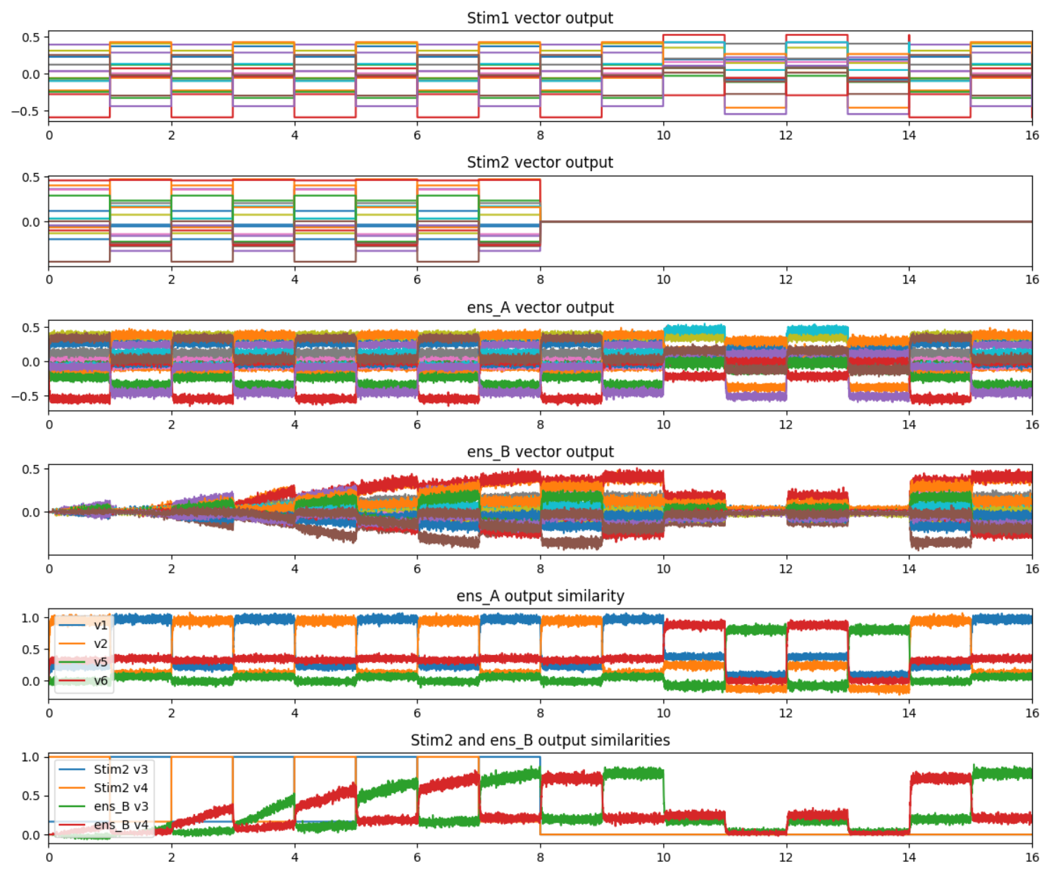
An error population is used to modulate the connection weights between A and B, with the PES learning rule set to train the network such that for a given x, the network output produces the vector y. After some period of training, the error population can be inhibited to stop the training process, at which point, the network output should be able to reproduce the x-y vector mapping. Here’s a graph of the network in action.
The graph above was produced by this code: example_pes.py (6.3 KB)
In the graph, the first half of the simulation (first 8 seconds) is the model’s training phase. After this, the learning is inhibited, and the network is presented with one presentation of the two vectors used in the training phase (v1 and v2). Next, two presentations each of two vectors novel to the model is shown. This is to demonstrate that for untrained vector inputs, the model doesn’t produce much of an output (as expected). Finally, two presentations each of the trained vectors are shown again, just to demonstrate that the learned weights are persistent, especially after the presentation of the untrained vector inputs. As mentioned above, the training phase is stopped by inhibiting the error population. The Stim2 output is zeroed out as well (this doesn’t affect the network though) just to show when the training has stopped.
Caveats of the PES network
There are a few caveats to note about the PES network.
- First, unlike your description, the
y vector doesn’t directly drive the B ensemble. Rather, the network is dependent on the PES learning rule to modulate the “communication channel” connection such that B produces the correct output.
- Second, you’ll notice that in the graph above, when the untrained vectors are presented to the model, the model still produces some (small) vector output. Depending on your use case, this may not be ideal. To rectify this issue, you’d want to apply the Voja learning rule to the
A ensemble (which essentially gives you the model you linked in your post)
- Third, this approach is technically “supervised”, since an
error population to modulate the learning rule. Although, I suppose this approach can be considered “unsupervised” if the entire model is treated as a black box which only needs x and y to train the association.
- Also note that I didn’t spend a lot of time tweaking the model, and improvements can probably be made to the learning rate and ensemble parameters to get a more accurate output.
- As for why the model is only trained for 8 seconds when a longer training phase would probably have benefitted the model, I wanted to match the STDP version of the model (which I created first), so I tweaked the parameters enough such that the 8 seconds of training had an acceptable output.
The STDP Approach
This approach uses the STDP code which I discussed in this forum post (also attached below). With this approach, the idea is to feed the A and B populations with the respective vector pairs, and use an STDP modulated connection between A and B to strengthen connections such that when the subset of A neurons that fire in response to x, the corresponding subset of B neurons also fire to reproduce y. With this approach, the network will look like this:
x --> A
      |
    (STDP)
      ↓
y --> B --> output
And here’s a graph of the network in action.
As with the PES example, the experiment layout is identical. The first half of the experiment is the training phase, then 2 presentations of trained vectors, 4 presentations of untrained vectors, then another 2 presentations of trained vectors. Because the STDP learning rule cannot be “switched off”, training is stopped by setting the output of Stim2 to nothing (all zeros).
Here’s the code that will reproduce the results above: example_stdp.py (6.3 KB)
You’ll require the custom STDP module (stdp.py (15.9 KB)) to run the code above (just put both files in the same folder).
Caveats to the STDP approach
While the STDP approach is more in line with your request (it’s purely unsupervised, and with B receiving direct input of y), the STDP approach comes with its fair share of caveats.
- First, the STDP learning is always on. In the graph above, this is evident as the output of
B continues to increase in magnitude even in the “testing” phase (compare t=8s-10s to t=14s-16s). In contrast, for the PES network, once the learning is inhibited, the outputs remain constant.
- Second, because both
y and the output of A is projected to B, in the training phase, the output of B essentially becomes 2*y (because it’s the reference y + the learned transformation y). In contrast, the PES network would only max out at y, and this may be more desirable considering your use case.
- Third, because the STDP rule is dependent on spike timings, it is most effective when the neurons are firing a lot. It is for this reason that I tested the model only with unit-length normalized vector pairs. Vector that are not unit length (especially vectors with small-ish magnitudes close to 0), may not cause the neurons to spike enough for the STDP to be effective and may necessitate using more neurons in the ensemble, increasing the learning rate, and/or increasing the maximum firing rate of the neurons (i.e., it’ll require a lot of experimentation to get working). In contrast, the PES method does not have this constraint (the example you linked in your post demonstrates this).
- Fourth, the STDP method is considerably slower to simulate than the PES method. This is because the STDP learning rule operates on the full connection weight matrix between
A and B (i.e., A.n_neurons * B.n_neurons weight elements), whereas the PES method operate on the decoder level (i.e., A.dimensions weight elements).
- Note that for this model (see the comments in the code), I had to use non-default intercept ranges for the neurons to get the network to work. This may cause weirdnesses when trying to use vectors with small magnitudes.
General Code Comments
If you run both example codes, you’ll notice that in both cases, the model is seeded with a random seed. This is just so that you can run the code and reproduce the exact results shown above. I encourage you to test the network without the seeds and observe their stability and effectiveness. From my own experimentation, the PES approach (without Voja) is more sensitive and less stable than the STDP approach. But I’d expect it to be much more stable if Voja is introduced into the model.
You should also note that the learning rates chosen are pretty sensitive to the model parameters (in both versions of the code). If you change the model parameters (number of dimensions, number of neurons, etc.) you’ll have to experiment with the code to find learning rates that will work best for you.