Dear @xchoo thank you for your prompt answer. Lets suppose the following example:
with nengo.Network(seed=0) as net:
net.config[nengo.Ensemble].max_rates = nengo.dists.Choice([100])
net.config[nengo.Ensemble].intercepts = nengo.dists.Choice([0])
net.config[nengo.Connection].synapse = None
neuron_type =nengo.LIF(amplitude = 0.01)
# this is an optimization to improve the training speed,
# since we won't require stateful behaviour in this example
nengo_dl.configure_settings(stateful=False)
# the input node that will be used to feed in input images
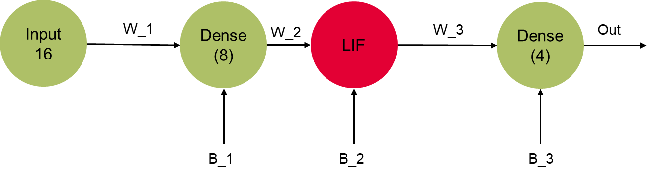
inp = nengo.Node(np.zeros(16))
x1 = nengo_dl.Layer(tf.keras.layers.Dense(8))(inp, shape_in=(1,16))
x1 = nengo_dl.Layer(neuron_type)(x1)
output = nengo.Probe(x1, label="output")
out = nengo_dl.Layer(tf.keras.layers.Dense(units=4))(x1)
out_p = nengo.Probe(out, label="out_p")
out_p_filt = nengo.Probe(out, synapse=0.01, label="out_p_filt")
When I print the weights before training:
Before training with get_nengo_params:
{'encoders': array([[ 1.],
       [ 1.],
       [ 1.],
       [ 1.],
       [-1.],
       [-1.],
       [-1.],
       [-1.]], dtype=float32), 'normalize_encoders': False, 'gain': array([2.0332448, 2.0332448, 2.0332448, 2.0332448, 2.0332448, 2.0332448,
       2.0332448, 2.0332448], dtype=float32), 'bias': array([1., 1., 1., 1., 1., 1., 1., 1.], dtype=float32), 'max_rates': Uniform(low=200, high=400), 'intercepts': Uniform(low=-1.0, high=0.9)}
Before training with sim.keras_model.weights:
[<tf.Variable 'TensorGraph/base_params/trainable_float32_8:0' shape=(8,) dtype=float32, numpy=array([1., 1., 1., 1., 1., 1., 1., 1.], dtype=float32)>, <tf.Variable 'TensorGraph/dense_25/kernel:0' shape=(16, 8) dtype=float32, numpy=
array([[-0.33486915,  0.40148127,  0.13097417, -0.06545389, -0.20806098,
         0.14250207,  0.4757855 , -0.06490052],
       [ 0.16010189,  0.10489583,  0.13663149,  0.11444879,  0.38933492,
         0.12776172,  0.03197503, -0.4740218 ],
       [-0.05912495, -0.24732924,  0.3862232 ,  0.38729346,  0.28728163,
        -0.44044805, -0.4289062 , -0.1915853 ],
       [-0.24881732,  0.4084705 , -0.02852035, -0.25761485,  0.13300395,
         0.08603108,  0.410012  ,  0.0701437 ],
       [-0.00356543,  0.0939151 ,  0.0414331 , -0.05708277, -0.20751941,
         0.23394465,  0.41970384,  0.16851854],
       [-0.28390443, -0.3134662 , -0.09283292, -0.49033797, -0.03442144,
        -0.20381367,  0.25012255,  0.02189696],
       [ 0.1371355 ,  0.06420732,  0.07077086, -0.47448373,  0.11151803,
        -0.1893444 , -0.01120353, -0.01354611],
       [-0.4414779 ,  0.39776003, -0.16403973,  0.41876316,  0.14977002,
         0.42905748, -0.07836056, -0.42671287],
       [ 0.26459813,  0.02045882, -0.33836246, -0.21259665,  0.18190789,
        -0.24045587, -0.40621114, -0.04324257],
       [ 0.30607176,  0.18740141,  0.21466279,  0.21725547, -0.30840743,
         0.17499697,  0.34543407, -0.20773911],
       [-0.40758514,  0.21844184, -0.20531535,  0.3941331 ,  0.2456336 ,
        -0.29453552,  0.28517365,  0.40464783],
       [-0.28130507,  0.21179736, -0.22052431, -0.40631115, -0.3692739 ,
        -0.34074497, -0.34367037,  0.34454226],
       [ 0.05650961,  0.03072739, -0.33571267, -0.33689427, -0.04421639,
        -0.15053117,  0.1564821 ,  0.4208337 ],
       [-0.39258194, -0.44293487, -0.22054589, -0.4338758 , -0.37818635,
        -0.04207456, -0.18798494, -0.03495884],
       [ 0.15310884,  0.15611696, -0.04791272,  0.39636707, -0.17005014,
        -0.279958  , -0.2546941 , -0.13452482],
       [-0.45635438, -0.22681558, -0.30091798, -0.16478252, -0.02208209,
        -0.23549163, -0.18475568, -0.08863187]], dtype=float32)>, <tf.Variable 'TensorGraph/dense_25/bias:0' shape=(8,) dtype=float32, numpy=array([0., 0., 0., 0., 0., 0., 0., 0.], dtype=float32)>, <tf.Variable 'TensorGraph/dense_26/kernel:0' shape=(8, 4) dtype=float32, numpy=
array([[ 0.01429349, -0.07985818, -0.12935376,  0.6964893 ],
       [ 0.26681113, -0.21800154, -0.09041494,  0.1429218 ],
       [-0.06134254,  0.3573689 , -0.44123855,  0.06895274],
       [ 0.06917661,  0.07004184, -0.31127587, -0.55301905],
       [ 0.18513662,  0.52865857,  0.04562682,  0.0864073 ],
       [-0.291421  ,  0.6059677 , -0.55191636,  0.6555473 ],
       [ 0.26294845, -0.30901057,  0.41675764, -0.56849927],
       [ 0.67330295,  0.47140473,  0.5104199 ,  0.23421204]],
      dtype=float32)>, <tf.Variable 'TensorGraph/dense_26/bias:0' shape=(4,) dtype=float32, numpy=array([0., 0., 0., 0.], dtype=float32)>]
After training the optimized weights are:
After training with get_nengo_params:
{'encoders': array([[ 1.],
       [ 1.],
       [ 1.],
       [ 1.],
       [-1.],
       [-1.],
       [-1.],
       [-1.]], dtype=float32), 'normalize_encoders': False, 'gain': array([2.0332448, 2.0332448, 2.0332448, 2.0332448, 2.0332448, 2.0332448,
       2.0332448, 2.0332448], dtype=float32), 'bias': array([0.99608827, 1.0442896 , 0.9583655 , 0.840119  , 0.8174738 ,
       0.9753371 , 1.1272157 , 1.1404463 ], dtype=float32), 'max_rates': Uniform(low=200, high=400), 'intercepts': Uniform(low=-1.0, high=0.9)}
After training with sim.keras_model.weights:
[<tf.Variable 'TensorGraph/base_params/trainable_float32_8:0' shape=(8,) dtype=float32, numpy=
array([0.99608827, 1.0442896 , 0.9583655 , 0.840119  , 0.8174738 ,
       0.9753371 , 1.1272157 , 1.1404463 ], dtype=float32)>, <tf.Variable 'TensorGraph/dense_25/kernel:0' shape=(16, 8) dtype=float32, numpy=
array([[-0.42222846,  0.24200168,  0.1228434 , -0.19200288, -0.21615249,
         0.22537254,  0.15830375,  0.14348662],
       [ 0.24897973,  0.24064443,  0.01594162, -0.01278597,  0.15329556,
         0.046916  ,  0.08096556, -0.27266836],
       [-0.47070235, -0.13800026,  0.347509  ,  0.11449179,  0.15270782,
        -0.66345483, -0.29918915, -0.1707631 ],
       [-0.5458111 , -0.04742003, -0.2862807 , -0.40992683,  0.25877243,
         0.07100935,  0.19473031,  0.14282067],
       [ 0.02363077,  0.4239431 , -0.01774568, -0.13983722, -0.3921473 ,
         0.29245335,  0.28123364,  0.0772593 ],
       [-0.47278467, -0.03457178, -0.14849444, -0.5372384 , -0.08720659,
        -0.32974714,  0.3656278 ,  0.07800148],
       [ 0.00100002, -0.3241698 ,  0.04821428, -0.43680564,  0.44487002,
        -0.18048719, -0.15704834,  0.13376418],
       [-0.5701078 ,  0.76006794, -0.22974566,  0.38979033, -0.09782179,
         0.38958353, -0.151282  , -0.47857407],
       [-0.04651041,  0.18091287, -0.41424903, -0.08234072,  0.2642943 ,
        -0.10087672, -0.45458052,  0.11325597],
       [ 0.21249026,  0.03274982,  0.3228077 ,  0.13583474, -0.36993992,
         0.3559691 ,  0.16389191, -0.16155171],
       [-0.51801544,  0.11881097, -0.08544519,  0.3828375 ,  0.0737737 ,
        -0.45559174,  0.09720748,  0.5586217 ],
       [-0.45184797,  0.18784086, -0.4561999 , -0.3188622 , -0.42621264,
         0.14698628, -0.55553156,  0.53076345],
       [-0.03956529, -0.10994054, -0.10967866, -0.3773059 , -0.24411117,
         0.03759727, -0.05840252,  0.36903772],
       [-0.41534385, -0.37392062, -0.26791674, -0.43218616, -0.5685533 ,
         0.10555435, -0.23374444,  0.01948378],
       [ 0.05834528,  0.2058212 , -0.2102371 ,  0.94866693,  0.12912013,
         0.20886466, -0.24586618,  0.02964282],
       [-0.4326087 , -0.35967124,  0.06181277, -0.40226054,  0.01146018,
         0.14308628, -0.4767727 , -0.09213054]], dtype=float32)>, <tf.Variable 'TensorGraph/dense_25/bias:0' shape=(8,) dtype=float32, numpy=
array([-0.00391253,  0.04429559, -0.04163574, -0.15988047, -0.18253754,
       -0.02466166,  0.12721722,  0.14045098], dtype=float32)>, <tf.Variable 'TensorGraph/dense_26/kernel:0' shape=(8, 4) dtype=float32, numpy=
array([[ 0.29734224, -0.04056702, -0.08777715,  0.3309865 ],
       [ 0.2889498 , -0.02732166, -0.20303652,  0.07589427],
       [ 0.3118579 ,  0.24252148, -0.542592  , -0.10831074],
       [ 0.11443946,  0.36353242, -0.6338987 , -0.592429  ],
       [ 0.11926413,  0.6897096 ,  0.03220635, -0.03515661],
       [-0.22724164,  0.48092696, -0.500028  ,  0.6807578 ],
       [ 0.00969276, -0.27644187,  0.5587347 , -0.4727213 ],
       [ 0.38449687,  0.6250343 ,  0.5408647 ,  0.32131493]],
      dtype=float32)>, <tf.Variable 'TensorGraph/dense_26/bias:0' shape=(4,) dtype=float32, numpy=array([-0.01315027, -0.02133778, -0.04621736,  0.10689242], dtype=float32)>]
You can see that the biases are changed when obtained with get_nengo_params compared to sim.keras_model.weights. But as you said that for efficiency the bias weights can get combined together to form one big matrix, considering this then if I have to put this neuron on the FPGA, what values I would use for the gain? By default, the gain of the LIF neuron is 1. Will I use the default values of the LIF neuron when a model with nengo_dl.Layer layers and trained with nengo_dl except for the bias that I will use the optimized one? or will I use the parameters I get with get_nengo_params. I hope I have explained my question well.
Thank you in advance for your answer.