While trying to use Nengo, I find that there are holes in my understanding of NEF. Therefore, I want to go back to some basics to see if it will help me in future with working with Nengo.
Basically, I am kind of getting that the NEF is a theory of explaining how biological neurons can represent mathematical values and perform computation. For representation, if we have a value \textbf{x} that we wish our neuron ensemble to represent, we can first convert it into a currents J(\textbf{x}) = \alpha_i e_i \textbf{x} + J_i^{bias}, before converting them into neuron activities a(t) = G[J(x)] where G is a nonlinear function.
However, I don’t think I fully understand what G and a(t) is. My current guess is that G is some function governed by the spiking neuron dynamics of:
\dot{V}(t) = \frac{1}{RC_m}(V + J(x)R - E_L)
Where E_L is the equilibrium potential. Therefore, there is no closed form of G unlike in ANN where we can describe some nonlinear Softmax or ReLU function.
I am not quite sure what a(t) is also and why it can be linearly multiplied and summed back to an approximation of the value \textbf{x} that we were trying to represent. Basically the NEF book just suggested that it can be done this way, but I wonder why it works.
That’s mostly correct. The NEF is a theory on how you can solve for the connection weights in order to get biological neurons to represent mathematical values and perform (approximate) mathematical computation.
That’s also correct, but I’d like to re-write the equations to clarify the formula. First,
That is to say, the input current to the i th neuron given some input vector \textbf{x} (i.e., J_i(\textbf{x})) is equals to the neuron gain (\alpha_i) multiplied by the dot product of the neuron’s encoder with the input vector (i.e., e_i \cdot \mathbf{x}) plus some bias current (J_i^{bias}).
Next,
a_i(\mathbf{x}) = G_i[J_i(\mathbf{x})]
That is to say, the activity (firing rate) of neuron i (a_i) is equals to this input current (J_i(\mathbf{x})) put through the neuron non-linearity G_i.
I will make two points here. First, the NEF does not place any limits on what G is. You can use the Softmax or ReLu non-linearities as the non-linear function G, and the NEF algorithm will still work the same (more on that later).
Secondly, for the LIF neuron, G is defined as follows (if you have the NEF book, it’s on page 37. See page 86 for the full derivation from the neuron membrane voltage equations):
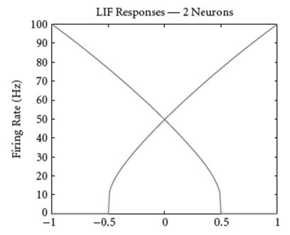
This is where the genius of the NEF algorithm comes in. From the equation above, we can compute the firing rate of the neuron for a specific input value \mathbf{x}. Now, let us suppose we sample random points covering the space from which we expect \mathbf{x} to get it’s values from (for a single dimensional input, this space defaults to values from -1 to 1; for multi-dimensional inputs, this space defaults to values within the unit hypersphere). For each random sample point of \mathbf{x}, we can compute the neuron activity a(\mathbf{x}), and we get a plot like this (this is for 2 neurons):
This is know as the neuron’s tuning curve, and for the plot above, these two neurons have been specifically configured (the gains and bias values are chosen specifically) so that they mirror each other.
Now, what the NEF algorithm does is it specifies a way to solve for a set of decoders (output weights) that you can apply to these tuning curves to get the desired output. Recall that the output of the ensemble is:
\hat{\mathbf{x}} = \sum_i a_i(\mathbf{x})d_i
That is to say, the output of the ensemble \hat{\mathbf{x}} is computed by multiplying the activity of each neuron with these (solved) decoders, and summing all of them up.
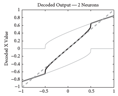
Let’s apply this to the two neurons from above. If we set the decoder of the neurons to roughly [0.85, -0.85], for each of the random samples of \mathbf{x}, we can compute the decoded output by multiplying the respective activity with the decoders. If we then plot it for all of the random samples, we get this:
Note that in the plot above, the decoded output is simply the weighted sum of the tuning curves.
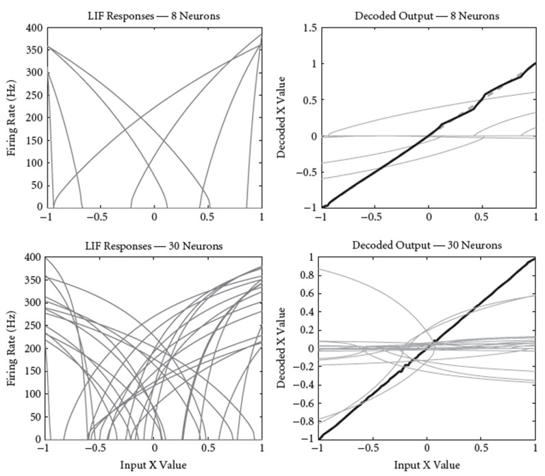
We can do the same process for ensembles with more neurons, and the more neurons we use, the better the approximation:
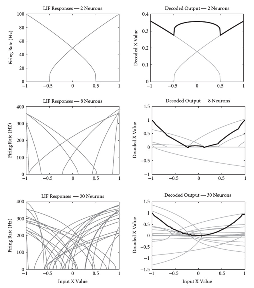
But the cool thing about the NEF is that if you change the function that you are trying to approximate, all it does is change the values of the decoders (i.e., changes the weighting of each tuning curve). The following is an example of using the exact same tuning curves as before, but modifying the NEF to approximate the function \hat{x} = x^2:
@xchoo, I think I finally get the math and intuition behind the NEF! The part about G[J] being able to take any form is especially a huge revelation for me. If I am not wrong, if we just treat G as a continuous function mapping current to activities a, this is just what everyone here refers to as a “rate” neuron and there is no spiking implementations right? But in the Nengo code, I also see spiking implementations with the dt parameter. I believe these are true spiking neurons that maps current to spike activities, and the rate neurons actually approximate these (or the other way round ).
Also, G seems differentiable even for LIF neurons, so is there a possibility that I can actually compute backpropagation for it?
So… the G formulation is what you get when you analytically solve the membrane voltage equations w.r.t. the input current. But, you can use those exact membrane voltage equations (since they specify the dynamics of how the membrane voltage evolves with input current) to get the output behaviour of a spiking neuron.
To relate spiking neurons to rate neurons (or the G equation), the activity you get with G is the steady-state firing rate of the spiking neuron given the same input current. There are a few caveats to this… First, because the simulation is discretized to a dt, it is possible that the resulting spikes (which have to align to dt) will cause the calculated spike rate to not match the rate-neuron’s rate. This can be solved by decreasing dt, or, doing things like allowing multiple spikes per timestep. There are other caveats involving discretization, such as you have to be careful when dealing with \tau_{ref} (e.g., the end of \tau_{ref} might be between two dts).
So, to answer your question, when dt approaches 0, the steady state of a spiking neuron will exactly match the rate activity given by G. The bigger dt gets (relative to the spike rate & \tau_{ref}), the more the spiking neuron becomes an approximation of the “true” activity that is given by G.
G is only differentiable when J(x) > J_{th}. When J(x) == J_{th}, you get in the denominator a ln(0) term, which is super nasty. In typical spiking neuron code, there’s usually some way of making sure that the computation doesn’t hit this singularity. This is the reason why LIF neurons can’t be directly used for backpropagation. But! You can slightly tweak the LIF activation function to make it differentiable at the singularity (basically you smooth out the singularity - see this paper). We call this neuron type the “SoftLIF” neuron and this is how NengoDL accomplishes training ANNs/SNNs with the LIF neuron.