This is still an active area of research and there is much to be understood, but I might as well display some partial results. Please note that this work is currently undergoing publication, and so please email me if you would like to use any of this or if you have any questions!
First bear with me as we set Denève’s networks to the side. We will instead start with the most basic recurrent NEF network imaginable: a 1D integrator, with no input, and using all of the defaults in Nengo:
import nengo
import nengolib
import numpy as np

import matplotlib.pyplot as plt
try:
    import seaborn as sns
except ImportError:
    pass

def go(n_neurons=30, perturb=0, perturb_T=0.001, T=10.0, dt=0.001,
       tau=0.001, tau_probe=1.0, seed=0, num_samples=10000):

    sample_every = max(T / float(num_samples), dt)

    with nengolib.Network(seed=seed) as model:
        stim = nengo.Node(output=lambda t: perturb if t <= perturb_T else 0)

        x = nengo.Ensemble(n_neurons, 1, seed=seed)
        nengo.Connection(stim, x, synapse=None)
        nengo.Connection(x, x, synapse=tau)

        p_voltage = nengo.Probe(x.neurons, 'voltage', sample_every=sample_every)
        p_x = nengo.Probe(x, synapse=tau_probe, sample_every=sample_every)

    with nengo.Simulator(model, dt=dt, seed=seed) as sim:
        sim.run(T)

    return sim.trange(dt=sample_every), sim.data[p_voltage], sim.data[p_x]
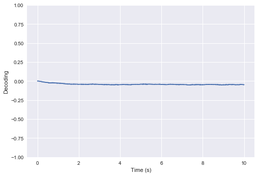
The ensemble will fluctuate around some stable decoded point, after a short transient period:
t, v1, x1 = go()

plt.plot(t, x1)
plt.ylabel("Decoding")
plt.xlabel("Time (s)")
plt.ylim(-1, 1)
plt.show()
Great, but now what will happen if we run it again with the exact same seed(s), and slightly perturbed initial conditions? More precisely, what happens if we make the input $10^{-15}$ for only the very first time-step, so that the initial voltage of each neuron becomes some extremely small epsilon (instead of zero)?
_, v2, x2 = go(perturb=1e-15)

plt.plot(t, x1)
plt.plot(t, x2)
plt.ylabel("Decoding")
plt.xlabel("Time (s)")
plt.show()
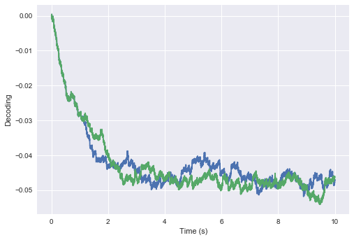
Curiously enough, the decoded value of each simulation starts off the same… but then after some short amount of time appears to spontaneously (and irreversibly) diverge!
For those who have studied chaotic systems, this should look extremely familiar as a hallmark behaviour of such systems (Strogatz, p. 328). To get a better intuition for what’s going on here, people will typically look at the trajectory of the “state” vector of the system, and measure the log L2-distance between the original trajectory and the perturbed trajectory at each point in time.
For this network, it makes the most sense (ignoring a few unimportant nuances) to consider the voltage vector of the population as the overall state. Below, we plot the log of the distance between the two trajectories from above:
plt.semilogy(t, np.linalg.norm(v1 - v2, axis=1))
plt.ylabel("Voltage Dist")
plt.xlabel("Time (s)")
plt.show()
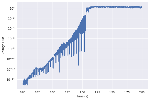
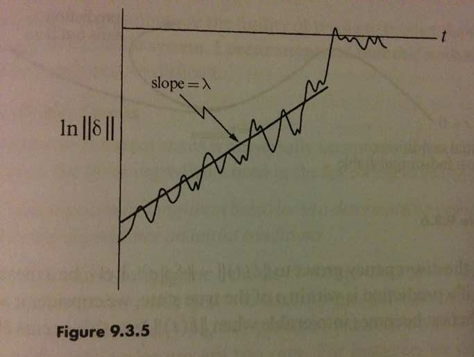
… which bears a striking resemblance to the same plots you get from your standard chaotic system (i.e., the Lorenz attractor):
What this means is that the distance between the two trajectories grows exponentially (up to the maximum possible distance on average). The slope of this plot is known as the Lyapunov exponent, which gives the exponential rate of divergence. Therefore, any amount of noise, no matter how small, will be amplified exponentially in time (a.k.a., the butterfly effect)!
But hold on… isn’t this just a linear integrator? Why are we getting nonlinear dynamics and chaos? Well the nonlinearities here are coming from the spiking neurons, which are nonlinear. All it takes is at least 3 dimensions and 1 nonlinearity to get chaos — here we have 30 of them.
More concretely, what we have here is actually known as a strange attractor. This is a special kind of chaotic system that evolves along a fractal manifold. The upper-bound on the distance is known as the diameter of this attractor. Each dimension of the attractor orbits predictably (in fact, this is given by the tuning curves at $x \approx 0$). But their phases shift chaotically with respective to one another. What the NEF is essentially doing then, from this perspective, is extracting order from within this chaos. The decoders (and synapse) extract useful information from the rate of each dimension’s orbit. This is made possible because the orbits themselves are predictable (for low-frequency inputs), which is analogous to the structure found in orbit diagrams and the Lorenz map (Strogatz, pp. 334-335, 360-367).
So, what does this have to do with the work of Sophie Denève and colleagues? My understanding is that this chaos is precisely what prevents their approach from scaling robustly when incorporating the biological details that come default with Nengo: most importantly, the refractory periods in the LIF model, and the non-zero lowpass filter on the feedback connection. Essentially, their methods rely on having a predictable trajectory for the voltage vector, in order to keep the state of the entire system under absolute control. Whether you can do this robustly depends on whether the network is in a chaotic or non-chaotic regime. If the network is chaotic, then any finite prediction error (no matter how small) will be amplified exponentially in time up to the diameter of the attractor. My understanding is that the situations with 1/N error scaling correspond to the regimes that are non-chaotic. Crucially, instantaneous feedback, without refractory periods, can be used to force the system into a non-chaotic regime. And, we don’t yet know if it is possible to relax any of these constraints without suddenly shifting back into chaos.
I won’t share @drasmuss code without permission, but I used it to verify that initial perturbations are not exponentially amplified in Denève’s networks. Rather, the distance persists with machine precision throughout the entire course of the simulation.
# arm_example is a modified verison of code from @drasmuss

def go_deneve(n_neurons=100, perturb=0, perturb_T=0.001, dt=1e-4, T=1, seed=0):
    rng = np.random.RandomState(seed)
    net = arm_example(n=n_neurons, dec_norm=0.03*(400.0/n_neurons),
                      rng=rng, seed=seed)
    with net:
        stim = nengo.Node(output=lambda t: perturb if t <= perturb_T else 0)
        p = nengo.Probe(net.ens.neurons, 'voltage')
        nengo.Connection(stim, net.ens[0], synapse=None)

    with nengo.Simulator(net, dt=dt) as sim:
        sim.run(T)

    return sim.trange(), sim.data[p]

t, v1 = go_deneve()
_, v2 = go_deneve(perturb=1e-3)

plt.semilogy(t, np.linalg.norm(v1 - v2, axis=1))
plt.ylabel("Voltage Dist")
plt.xlabel("Time (s)")
plt.show()

This indicates that this particular Denève-style network is operating in a non-chaotic regime. The trajectory of the voltage vector is entirely predictable, in that any noise / perturbations are not amplified in time.
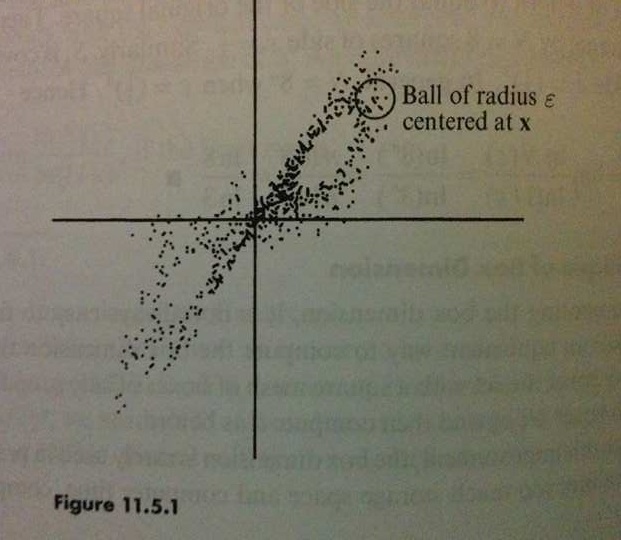
Returning to the NEF network, it may be of interest to some that we may numerically estimate the fractal dimension of the strange attractor (Strogatz, pp. 418-419). Disclaimer: these numerical measurements should always be taken with a grain of salt.
With 30 neurons, the dimension is about ~6.237. Essentially this means that the 30-dimensional neural activities are in fact tracing out a ~6.237-dimensional fractal.
t, v, x = go(T=500)

def correlation_dimension(v, size=100, powers=np.linspace(0, 10., 40)):
    """Correlation dimension from Grassberger and Procaccia (1983)."""
    n, d = v.shape
    v_sample = v[np.random.choice(n, size=size, replace=False)]

    eps = np.sqrt(n) * np.exp(-powers)
    data = np.zeros_like(eps)

    for v_i in v_sample:
        dist = np.linalg.norm(v - v_i[None, :], axis=1)
        for i in range(len(eps)):
            data[i] += np.count_nonzero(dist <= eps[i])
    data /= len(v_sample)

    return np.log(eps), np.log(data)

X, Y = correlation_dimension(v)

i = 17  # manually set to upper index of relevant tangent
j = 21  # manually set to lower index of relevant tangent

pylab.figure()
pylab.title((Y[j] - Y[i]) / (X[j] - X[i]))
pylab.plot(X, Y)
pylab.plot((X[i], X[j]), (Y[i], Y[j]), linestyle='--', lw=5, c='r')
pylab.xlabel(r"$\log \, \epsilon$")
pylab.ylabel(r"$\log \, N(\epsilon)$")
pylab.show()
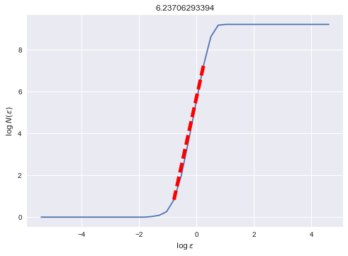
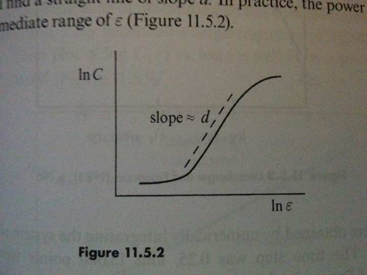
Finally, it is reassuring that the shape of this curve is typical of strange attractors:
Figures photographed from [*] Strogatz, Steven H. Nonlinear dynamics and chaos: with applications to physics, biology, chemistry, and engineering. Second Edition. Westview press, 2014.