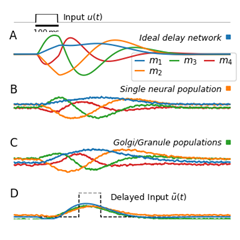
I am implementing the “ideal mathematical model” part of this article, but the results achieved are not ideal. I want to know what is wrong with my program. If you can solve my doubt, I would be very grateful!
import numpy as np
import matplotlib.pyplot as plt

q = 6
theta = 0.4
number_of_points = 100


def get_a_and_b():
    # A:
    a = np.zeros([q, q])
    for i in range(q):
        for j in range(q):
            if i < j:
                a[i, j] = (2 * i + 1) * -1
            else:
                a[i, j] = (2 * i + 1) * ((-1) ** (i - j + 1))
    # B:
    b = np.zeros(q)
    for i in range(q):
        b[i] = (2 * i + 1) * ((-1) ** i)
    return a/theta, b/theta


if __name__ == "__main__":
    A, B = get_a_and_b()

    m = np.zeros(q)
    output = np.zeros([number_of_points, q])

    for i in range(number_of_points):
        if i < 10:
            u = 1
        else:
            u = 0
        B_u = u * B
        m = m + np.dot(A, m) + B_u
        output[i, :] = m

plt.plot(range(number_of_points), output)
plt.show()
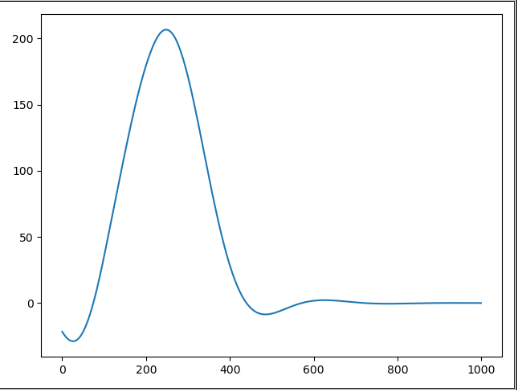
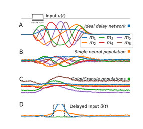
There is an important distinction here between continuous-time dynamics and discrete-time dynamics. From your code it looks like you are trying to implement equation 1 from this paper (@astoecke, @tcstewar). That equation is a continuous-time dynamical system, in that $Am + Bu$ corresponds to an instantaneous derivative at the current moment in time ($\dot{m}(t)$). It does not correspond to a discrete change ($m[t] \rightarrow m[t + \Delta t]$).
When you do m = m + np.dot(A, m) + B_u you are implementing a discrete-time dynamical system, with some discrete update across some time-step. In fact, you are applying the Euler method with a time-step of $\Delta t = 1$ unit of time. And since you have $\theta = 0.4$ units of time, you are attempting to do an Euler update that is more than double the time-scale of the dynamical system. That will give you an unstable discretization of the system.
One solution is to do Euler’s method with a time-step that is much smaller than theta. For example,
dt = 1e-3
m = m + dt*(np.dot(A, m) + B_u)
and then simulate the system for 100,000 time-steps rather than 100 time-steps.
Another solution is to use a stable discretization method such as zero-order hold (ZOH). Here is an example of how you can do it using scipy.signal with $\Delta t = 0.01$. There will also be support for this system in an upcoming release of Nengo. Modified version of your code:
import numpy as np
import matplotlib.pyplot as plt
import scipy.signal

q = 6
theta = 0.4
number_of_points = 100


def get_a_and_b():
    # A:
    a = np.zeros([q, q])
    for i in range(q):
        for j in range(q):
            if i < j:
                a[i, j] = (2 * i + 1) * -1
            else:
                a[i, j] = (2 * i + 1) * ((-1) ** (i - j + 1))
    # B:
    b = np.zeros(q)
    for i in range(q):
        b[i] = (2 * i + 1) * ((-1) ** i)
    return a/theta, b/theta


Acont, Bcont = get_a_and_b()

# Discretize the dynamical system using ZOH
dt = 0.01
Adisc, Bdisc, _, _, _ = scipy.signal.cont2discrete(
    (Acont, Bcont[:, None], np.zeros((1, q)), 0),
    dt=dt,
    method='zoh',
)
Bdisc = Bdisc.squeeze(axis=1)

m = np.zeros(q)
output = np.zeros([number_of_points, q])

for i in range(number_of_points):
    if i < 10:
        u = 1
    else:
        u = 0
    m = Adisc.dot(m) + Bdisc * u
    output[i, :] = m

plt.plot(range(number_of_points), output)
plt.show()
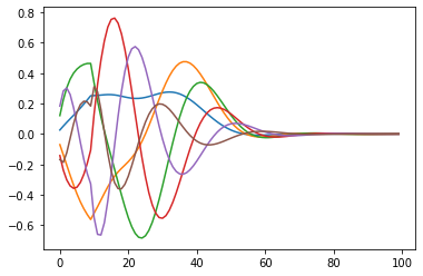
Note that the polynomials decay back to zero around time-step 50, because $\theta / \Delta t$ = $0.4 / 0.01 = 40$ in this example, and the input goes to zero at time-step 10 (so, 10 + 40 = 50). At each moment in time, these polynomials give a reconstruction of the last 40 time-steps. More information can be found on this system in this NeurIPS paper and a deep learning Keras implementation is available at https://github.com/nengo/keras-lmu.
Thank you very much for your quick and detailed answers, which helped me solve this problem! By the way, in the paper, I saw that Figure 3(A) can be output as Figure 3(D) through decoding, so how is the decoding vector set? I used Legendre polynomial to decode, but the result seems to be wrong.
import numpy as np
import matplotlib.pyplot as plt

q = 6
theta = 0.4
number_of_points = 10000
dt = 1e-4


def get_a_and_b():
# A:
    a = np.zeros([q, q])
    for i in range(q):
        for j in range(q):
            if i < j:
                a[i, j] = (2 * i + 1) * -1
            else:
                a[i, j] = (2 * i + 1) * ((-1) ** (i - j + 1))
# B:
    b = np.zeros(q)
    for i in range(q):
        b[i] = (2 * i + 1) * ((-1) ** i)
    return a/theta, b/theta


def legendre(x, order):
    if order is 0:
        return 1
    elif order is 1:
        return x
    else:
        a = (2 * order - 1) * x * legendre(x, order - 1)
        b = (order - 1) * legendre(x, order - 2)
        return (a - b) / order


def encoder():
    A, B = get_a_and_b()

    m = np.zeros(q)
    output = np.zeros([number_of_points, q])

    for i in range(number_of_points):
        if 1000 < i < 2000:
            u = 1
        else:
            u = 0
        B_u = u * B
        m = m + dt * (np.dot(A, m) + B_u)
        output[i, :] = m

    return output


def decoder(m):
    output = np.zeros(number_of_points)
    width = int(theta / dt)
    for t in range(number_of_points):
        print(t)
        for i in range(width):
            if t - i < 0:
                break
            o = 0
            for n in range(q):
                o = o + m[t][n] * legendre(i / width, n)
            output[t - i] += o
    return output


if __name__ == "__main__":
# encoder
    output = encoder()
    output2 = decoder(output)

    plt.plot(range(number_of_points), output2)

    plt.show()
There’s an easier way to construct the Legendre polynomials using scipy.special.legendre. You can use this to create a vector of polynomials (evaluated at the points you want to reconstruct), and then apply them with a dot product, like so:
def decoder(m, points_to_reconstruct=2):
    output = np.zeros(number_of_points)
    width = int(theta / dt)
    window = np.linspace(0, 1, points_to_reconstruct)
    D = np.asarray([legendre(i)(2 * window - 1) for i in range(q)])
    return m.dot(D)
This decodes a two-dimensional array, where the first element is an approximation of u(t) and the second is an approximation of u(t - theta). Increasing the value of points_to_reconstruct gives you evenly spaced points in between. You can also replace np.linspace(0, 1, points_to_reconstruct) with whatever points you want within the window (normalized to [0, 1]).
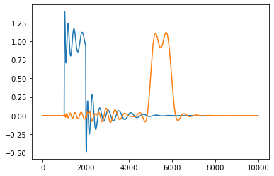
However, one thing to note is that the reconstruction is approximating the window using polynomials up to order q - 1. If you have a step function, such as the one in your example, then it is impossible for a finite number of polynomials to fit such a curve, as it has discontinuous derivatives wherever there are discontinuous changes in the input (whereas, in contrast, polynomials have continuous derivatives). You do better if you increase q, though, in the same way that higher-order Taylor series form better approximations as you add more polynomials to the series.
In general, the reconstruction will work best for low-frequency inputs, where the frequency scales linearly with q. That is, if you double the frequency of your input signal, then you need twice as many polynomials to fit it as accurately.
Here’s an example taking your previous code, increasing q to 24, using ZOH discretization, and the above decoder function:
import numpy as np
import matplotlib.pyplot as plt
import scipy.signal
from scipy.special import legendre

q = 24
theta = 0.4
number_of_points = 10000
dt = 1e-4


def get_a_and_b():
# A:
    a = np.zeros([q, q])
    for i in range(q):
        for j in range(q):
            if i < j:
                a[i, j] = (2 * i + 1) * -1
            else:
                a[i, j] = (2 * i + 1) * ((-1) ** (i - j + 1))
# B:
    b = np.zeros(q)
    for i in range(q):
        b[i] = (2 * i + 1) * ((-1) ** i)
    return a/theta, b/theta


def encoder():
    Acont, Bcont = get_a_and_b()

    Adisc, Bdisc, _, _, _ = scipy.signal.cont2discrete(
        (Acont, Bcont[:, None], np.zeros((1, q)), 0),
        dt=dt,
        method='zoh',
    )
    Bdisc = Bdisc.squeeze(axis=1)

    m = np.zeros(q)
    output = np.zeros([number_of_points, q])

    for i in range(number_of_points):
        if 1000 < i < 2000:
            u = 1
        else:
            u = 0
        # B_u = u * B
        # m = m + dt * (np.dot(A, m) + B_u)
        m = Adisc.dot(m) + Bdisc * u
        output[i, :] = m

    return output


def decoder(m, points_to_reconstruct=2):
    output = np.zeros(number_of_points)
    width = int(theta / dt)
    window = np.linspace(0, 1, points_to_reconstruct)
    D = np.asarray([legendre(i)(2 * window - 1) for i in range(q)])
    return m.dot(D)


output = encoder()
output2 = decoder(output)

plt.plot(range(number_of_points), output2)

plt.show()
Note the ringing around the edges occurs from the higher-order polynomials trying to fit the instantaneous changes in the input. It would look much better with a filtered or low-frequency input.
Thank you very much for your answer! I am very interested in this article, I found its poster and saw the corresponding Github project. But unfortunately, this website cannot be accessed. May I ask, is the website I visited wrong? https://github.com/ctn-waterloo/cogsci2020-cerebellum
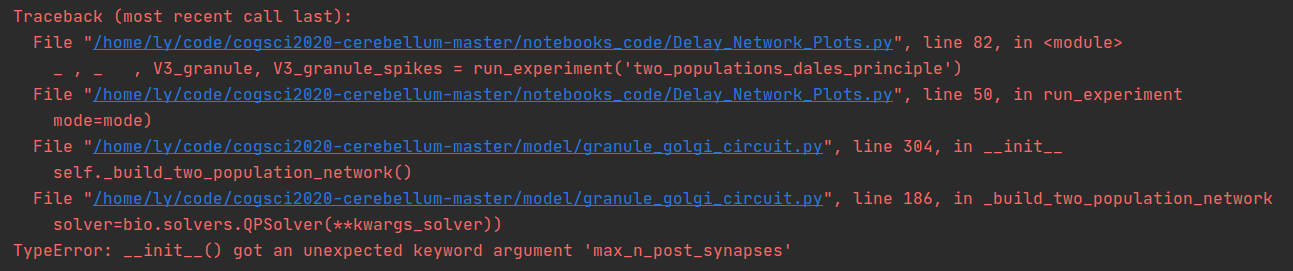
Thank you very much for your answer! But I encountered some problems when running this program. What is the problem?I would be very grateful if you can answer my question
Operating environment:
Ubuntu 18.04
python 3.6.6
nengo 3.1.0
Hm, did you make sure that you are running a version of NengoBio from the end of January 2020 as stated in the readme? The code is as it was back when we submitted the paper, and I haven’t updated it to work with newer versions of NengoBio, which no longer feature the max_n_post_synapses parameter.
I think that the latest version of NengoBio that should be compatible with this code is Git commit 8ff2274f8f5e09877ed0a554ca268f9fa396e3a5. You can simply checkout that commit from the NengoBio Git repository and install it from there by running pip3 install -e .. Make sure to uninstall any currently installed NengoBio version before you do that.
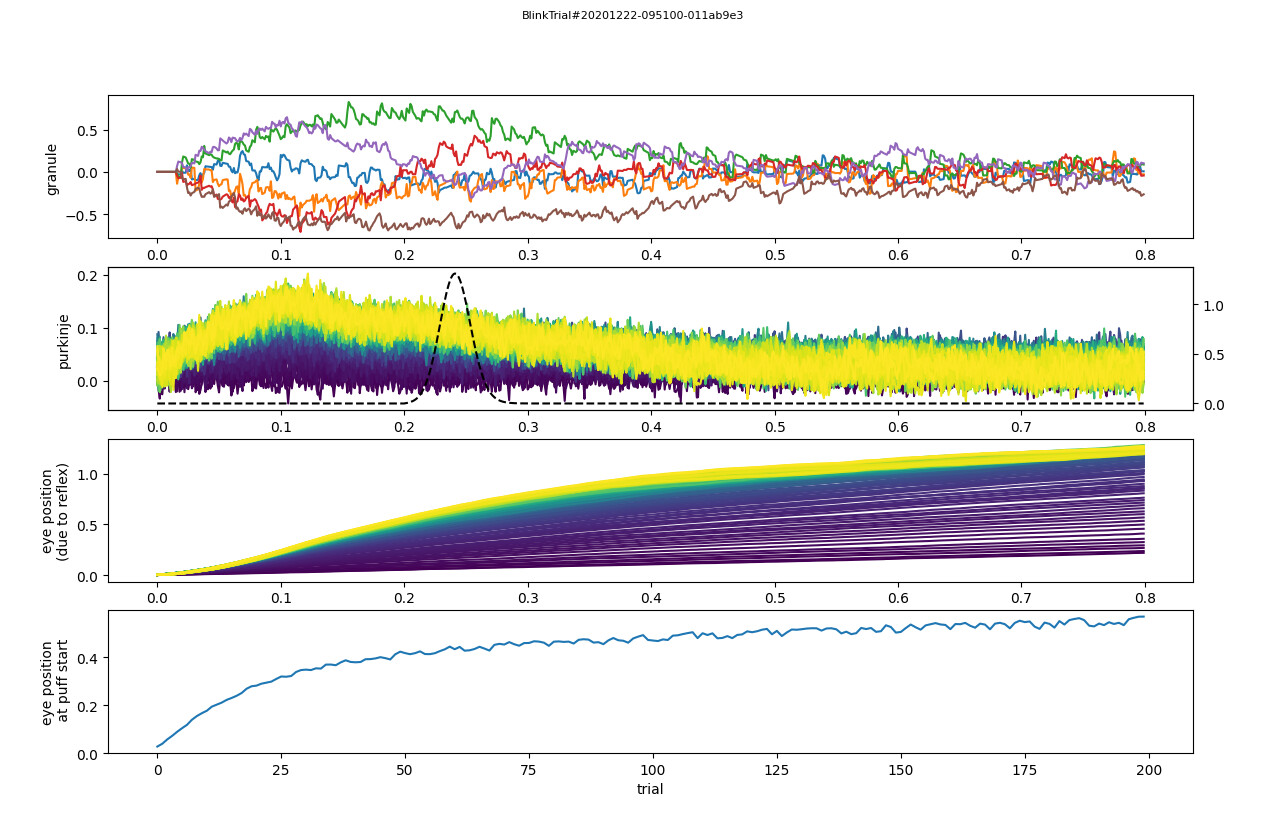
When I was running the model exploration file in the notebook, I found that the running result was different from the expected result. Could it be my mistake? I have been thinking about this issue for some time, I would be very grateful if I can get your advice.
I think that your results are exactly what they should be. The committed version of the notebook was executed on Jan 22, and the default parameters model changed quite significantly since then. If you revert back to the Jan 22 revision 79b4fb5d48a5feb91eef15e02bc356d093160a59 (and revision 37a5e17d4b62a495e46fb21af0d55b07d7bf5e15 of nengo-bio) you will get the results that were stored in the notebook.
Edit: As the name of the notebook suggests, we only used this notebook for playing around with the model. The data shown there are not what we reported in the paper. We used the notebook Run Model.ipynb for that, which I apparently didn’t commit until Apr 2. It thus wasn’t included in the repository that I uploaded to GitHub. I have now added Run Model.ipynb.
Thank you very much for your detailed guidance, my problem has been solved. But there is another question that has always puzzled me. Is there any basis for setting q=6 in the paper? I tried q=4 and q=10, and the results they achieved are as follows:
I would be very grateful if you can answer my doubts!At the same time any suggestions or ideas are welcome!
Excellent question! We don’t really discuss this in the paper. There are two reasons, really.
The dynamical system becomes unstable for larger $q$ when building the Granule-Golgi circuit, as you have noticed. $q = 6$ is kind of a compromise between being stable and having a sufficiently good temporal basis. We are not exactly sure where the instabilities come from, but we think that it has to do with the higher frequencies of some of the state dimensions.
As Voelker and Eliasmith show in their 2018 Neural Computation paper [1] the Delay Network matches time cell data from the brain for $q = 6$, but not for other dimensionalities.
Thank you for your detailed and patient answer!
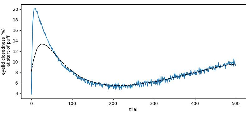
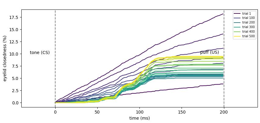
In the paper I saw that you used the data from Heiney et al. (2014), but I did not find his experimental data in his paper or appendix. Is his data public? Would you share his data or the way to obtain the data with me please?In addition, how does your paper model the 6 mouse models? There are ANTAGONIST and AGONIST in the code. Is this used to model different mouse models? Is there a basis for setting the values of ANTAGONIST and AGONIST?
That data is in the paper in the form of diagrams. We manually digitized the diagrams to get the data (our extracted data points should be in one of the notebooks). We (very roughly) fitted the motor model to the eyeblink trajectories reported in one of the papers.
Thank you for your answer. I searched the notebook carefully and did not find the data points you extracted based on the paper (Heiney et al.(2014)). Could you tell me the exact path of the data in the notebook?
In your paper, the eyeblink trajectories of 6 rats is simulated. Did you fit the data based on the eyeblink trajectories of different rats?
Ah, the traced diagrams were in the experimental_data folder, which I originally didn’t upload to GitHub because it contained tons of copyrighted material. I’ve cleaned that folder up and uploaded it to GitHub. The data are loaded at the beginning of Plot - Results - Basic.ipynb.
Regarding to the motor system parameters, I’ve added my original notebook Eyeblink Motor System.ipynb to the repository; I’m noting therein which paper and which figure I fitted the data to.
We’re using the same set of motor system parameters for all experimental trials.
Thanks a million. Now I have plotted the neurobiological data, but in the process of running plot-result-basic, I regret that I did not reproduce the model data in the paper. Is it because I am using the wrong software package or code version?
nengo-bio: commit 8ff2274f8f5e09877ed0a554ca268f9fa396e3a5
cogsci2020-cerebellum-master: f0f14a66a4d6210c6e513e67982acbaa06532bbe
System:Ubuntu18.04
Interesting; I just used this code last week and I’m getting exactly the same results we got last year. How exactly did you generate the data that you’re visualising here, i.e., can you provide me with a step-by-step list of things that you do to produce these figures (starting with a fresh copy of the repository)?


 Now I have plotted the neurobiological data, but in the process of running plot-result-basic, I regret that I did not reproduce the model data in the paper. Is it because I am using the wrong software package or code version?