Problems with inference

Hi,
I’m learning Nengo-DL and am stuck at a very basic thing. I want to create a network that predicts a number of signals.
I’m following the tutorials https://www.nengo.ai/nengo-dl/examples/tensorflow-models.html.
So I built a basic autoencoder model in Keras, which works. Then I changed it into Nengo Ensembles with RectifiedLinear neurons and it still works. But when I try to use spiking neurons the training looks successful and prints decreasing loss values, but I can’t find a way to get a prediction on test data. All I get is a constant value for all input dimensions.
My code looks like:

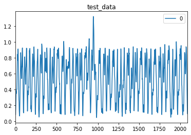
# train_data, validation_data, test_data are arrays [timesteps, features]
train_data = train_data[:, None, :]
validation_data=validation_data[:, None, :]
test_data = test_data[:, None, :]


earlyStopping= EarlyStopping(monitor='val_loss', patience=3, verbose=2,  min_delta=1e-4, mode='auto')
lr_reduced = ReduceLROnPlateau(monitor='val_loss', factor=0.5, patience=1, verbose=2, min_delta=1e-4, mode='min')

with nengo.Network(seed=seed) as net:
    # set up some default parameters to match the Keras defaults
    net.config[nengo.Ensemble].gain = nengo.dists.Choice([1])
    net.config[nengo.Ensemble].bias = nengo.dists.Choice([0])
    net.config[nengo.Connection].synapse = None
    net.config[nengo.Connection].transform = nengo_dl.dists.Glorot()
#     # parameters for spiking neurons
    net.config[nengo.Ensemble].max_rates = nengo.dists.Choice([100])
    net.config[nengo.Ensemble].intercepts = nengo.dists.Choice([0])
    net.config[nengo.Connection].synapse = None

    inp = nengo.Node(output=np.ones(X1.values.shape[-1]))

    #layers_sizes is a list of the layers' last dimension sizes
    l = inp
    for ls in layers_sizes:
        hidden = nengo.Ensemble(100, ls 
#                                 ,neuron_type=nengo.RectifiedLinear()
                                ,neuron_type=nengo.LIF(amplitude=0.01)
                               ).neurons
        nengo.Connection(l, hidden)
        l = hidden

    #the last layer without any activation
    #I could not find a way to do it within nengo, so just adding a TF layer :-)
    out = nengo_dl.Layer(
        tf.keras.layers.Dense(ls))(l)

    out_p = nengo.Probe(out, label="out_p")
    
with net:
    nengo_dl.configure_settings(stateful=False, use_loop=False)

# when testing our network with spiking neurons we will need to run it
# over time, so we repeat the input/target data for a number of
# timesteps.
n_steps = 30
test_data = np.tile(test_data, (1, n_steps, 1))

sim = nengo_dl.Simulator(net, minibatch_size=32)

sim.compile(optimizer=tf.optimizers.Adam(lr=0.001),
            loss='mean_squared_error')

sim.fit(train_data, train_data,
        epochs=500,
        batch_size=32,
        shuffle=False,
        callbacks = [earlyStopping, lr_reduced],
        verbose = 2,
        validation_data=(validation_data, validation_data))

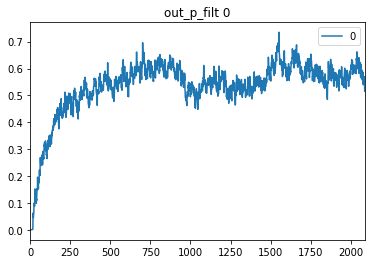
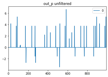
preds = pd.DataFrame(data=sim.predict(test_data)[out_p][:,0,:])
preds.plot()

I’m struggling with this for a few days now, please help!

Hello @mkravchik1 and welcome! If you change LIF to LIFRate does the problem go away? If so, it would seem that the neurons are rarely (if at all) spiking. You could confirm this by adding probes of the form nengo.Probe(hidden.neurons, 'spikes') to probe the spiking activity of those hidden layers. My best guess is that the neurons in later layers are not spiking, due to the firing rates of the trained network being close to zero.

One ‘warning’ to me is that you are setting both (gain, bias) and (max_rates, intercepts), where the latter is redundant when you set the former. The simulator should be issuing you a warning about this when you first initialize nengo_dl.Simulator(net, ...), of the form:

NengoWarning: Specifying the gains and biases for <Ensemble (unlabeled) at 0x7f3e0a2be908> imposes a set of maximum firing rates and intercepts. Further specifying either max_rates or intercepts has no effect.

This means that the initial gains of your neurons will end up being 1, which is quite low for the default spiking LIF neuron. You could try first switching to SpikingRectifiedLinear and choosing a larger initial gain such as 100 (which would correspond to a firing rate of 100 Hz for an input current of 1 and a time-step of 1 ms).

One more important thing. I noticed you’re only probing the first time-step of the output ([:,0,:]), but you will need to simulate the SNN for a few time-steps in order to get a response from the output layer. You may want to add some synapses to at least your output probe to filter the spikes, and allow enough time for the neurons to spike and for those spikes to be filtered. If your input is static, then the would want to repeat them (hold them constant) across the time axis for the chosen number of time-steps. See here for an example: https://www.nengo.ai/nengo-dl/examples/spiking-mnist.html

Hi @arvoelke and thank you! I tried switching to LIFRate, but do not see any change. I removed setting max_rate and intercepts, but this has not changed anything.

I increased the number of tiled test_data to 1000 but again no change.
When I try to add another probe, either to the hidden layers or to the output one I can the following error on the call to fit:
ValueError: No data provided for "out_p". Need data for each key in: ['lh_spikes', 'out_p']

or

ValueError: No data provided for "out_p_filt". Need data for each key in: ['out_p', 'out_p_filt']

Why I see those?

Also, I looked at the output I get from predict, it has only 1 timestamp, so it does not matter whether I use [:,0,:] or [:,-1,:]

Lastly, I switched to SpikingRectifiedLinear neuron, but then the network does not converge during training.
Seems I’m missing some basic understanding, but I’ve went through both Nengo and Nengo-DL tutorials and can’t figure this out.
Please advice, I really have no idea where to go from here.

Hi @arvoelke,
I made some progress myself, answering some of my own questions.

  1. The error message about additional Probes was caused by the loss function that was not targeting a specific probe, but all of them. I fixed it by using:
    sim.compile(optimizer=tf.optimizers.Adam(lr=0.001), loss={'out_p':'mean_squared_error'})

and
sim.fit(x={inp:train_data},
y={‘out_p’:train_data},

2. Another source of this error was the validation data. I haven’t found how to tell Nengo/Keras that is should be applied only to the out_p probe, so for now I just removed it from fit arguments
3. I was able to see that indeed the neurons don’t spike. So I removed the gain and bias initialization and now the neurons seem to be firing. It even decreased the training error I’m getting from fit.

However, when I try to get the prediction I still don’t see anything resembling the test_data.
What I do is:
n_steps = 300
test_data = np.tile(test_data, (1, n_steps, 1))
sim.run_steps(n_steps=n_steps, data={inp:test_data[:minibatch_size,:,:]})

I’d like to ask a number of best-practice questions:

  1. If I want to model and predict time-series data should I pass it as [batches, timesteps, dimensions] or as [timesteps, 1, dimensions]. The latter was the format i used in Keras adaptation to Nengo.
  2. I’m confused about reading the model’s output with spiking neurons. My model should terminate with a dense layer without any activation. I haven’t found any direct implementation of this in Nengo and used a wrapper around tf.keras.layers.Dense. So when I read its output should I see spikes trains and low-filter them to get the predicted value, or should I see a value that I can directly compare to the expected output (neither works for me as of now)?
    Is there any example of nengo-dl predicting multivariate timeseries?
    Thanks a lot!

In the process of writing up this reply I noticed another thing about your code. Where you have:

hidden = nengo.Ensemble(100, ls, ...) 
nengo.Connection(l, hidden)
l = hidden

I think you instead want:

hidden = nengo.Ensemble(ls, 1, ...)
nengo.Connection(l, hidden.neurons)
l = hidden.neurons

in order to directly connect all of the neurons to eachother with weight matrices. The first approach connects them in a latent space represented by layers of only 100 neurons (using factored matrices with ls latent dimensions), which I’m guessing is not what you want given that you’ve named the ls variables layers_sizes. The second approach uses ls neurons and learns full matrices between layers (note the value 1 is ignored in this case).

Great. Glad that was figured out.

It should work to call:

sim.fit(
    x={'inp': train_data},
    y={'out_p': train_data},
    validation_data=(validation_data, validation_data),
    ...
)

Let us know if this is not working or if you get an error message. However, as a quick check, do you want to be using the same data for both the input and the output? This is effectively training the network as an auto-encoder (regenerate the output given the input). So just making sure this is what you want to be doing.

How are you looking at the predictions? Are you using a filtered probe, like out_p_filt with e.g., synapse=0.1 from the link I provided?

If your data is a time-series, and you want each input to be a sequence that is provided to the model one step at a time, then it should be shaped as [batches, timesteps, dimensions] where timesteps is the number of steps in the time-series. I feel that this might be where some of the understanding issues might be coming from. Spiking neurons and synapses need to be simulated over time, and the network will have internal state that changes from one step to the next according to the time-series that you provide in this middle axis.

The Dense layer approach is fine assuming its output shape matches your output data.

The output will be spike trains that have been weighted together by some linear combination of weights. Lowpass filtering them (e.g., with synapse=0.1 on the probe) will also average them together over time (e.g., for synapse=0.1 and the default time-step of dt=0.001 it will integrate them on the order of roughly 100 time-steps) to filter out the high-frequency noise in the spikes.

Assuming it is training okay, the filtered output probe will be a lowpass filtered version of your desired output. The unfiltered probe will be a noisy version. You can make it less noisy by adding more neurons, or by adding a filter.

https://www.nengo.ai/nengo-dl/examples/lmu.html

There’s this example that provides MNIST sequentially as a permuted one-dimensional time-series (known as the psMNIST benchmark for RNNs). However it is not using spiking neurons. This paper explains how to train it as a spiking network (in review): https://arxiv.org/abs/2002.03553 – code will be released after review.

Thank you very much for guiding me!

Actually, I started like this, but then I read the tutorial 07-multiple-dimensions.py and understood from there that the input signal’s features are represented by the dimensions parameter and the n_neurons control how many neurons I average to represent these dimensions. I indeed want to build multivariate time series autoencoder, thus each layer will have different number of features (code size or layer size). So was my understanding wrong?

Nope, I still get an error message.

Yes, exactly. I put this probe on the last Dense layer. The results look quite differently from the test_data which I’m trying to reconstruct.

Just to make sure I - if I have one long time-series with N timesteps in it, should I feed it as
[1, N, dimensions]? In that case, will the network run for exactly N steps and its output be the reconstruction of the input signal (in my case of autoencoder)? Or do I need to run it for more steps and use the last N?

I will study the references you sent. Would appreciate if you could relate to my questions above, because I seem to do what you suggested and still the filtered output is not what I expect. When I switched to the nengo.Ensemble(ls, 1, ...) the output is still not resembling the reconstructed data.
Thank you so much!

Just to clarify, my current code looks like this:

# split into training and validation
X1, X2, _, _  = train_test_split(X, X, test_size=0.33, shuffle=False)

with nengo.Network(seed=seed) as net:
    net.config[nengo.Connection].synapse = None
    net.config[nengo.Connection].transform = nengo_dl.dists.Glorot()
    net.config[nengo.Ensemble].max_rates = nengo.dists.Choice([100])
    net.config[nengo.Ensemble].intercepts = nengo.dists.Choice([0])

    inp = nengo.Node(output=np.ones(X1.values.shape[-1]))
    
    l = inp
    for ls_idx, ls in enumerate(layers_sizes):
        hidden = nengo.Ensemble(n_neurons=ls*2, dimensions=ls 
                                ,neuron_type=nengo.LIF(amplitude=0.01)
                               ).neurons
        nengo.Connection(l, hidden)
        l = hidden
        p_spike = nengo.Probe(l, label="p_spike_%d"%ls_idx)
        
    #the last layer without any activation
    #I could not find a way to do it withing nengo, so just adding a TF layer :-)
    out = nengo_dl.Layer(
        tf.keras.layers.Dense(ls))(l)

    out_p = nengo.Probe(out, label="out_p")
    out_p_filt = nengo.Probe(out, synapse=0.1, label="out_p_filt")
with net:
    nengo_dl.configure_settings(stateful=False, use_loop=True)


train_data = X1.values[None, :, :]
validation_data=X2.values[None, :, :]
test_data = X4.values[None, :, :]

minibatch_size=64

#resize the data
def resize_to_batches(data, minibatch_size):
    features = data.shape[-1]
    data = data[:,:data.shape[1]//(minibatch_size)*minibatch_size,:]
    data = data.reshape((minibatch_size, -1, features))
    return data

train_data = resize_to_batches(train_data, minibatch_size)
sim = nengo_dl.Simulator(net, minibatch_size=minibatch_size)

sim.compile(optimizer=tf.optimizers.Adam(lr=0.001),
            loss={'out_p':'mean_squared_error'})

sim.fit(x={inp:train_data}, 
        y={'out_p':train_data},
        epochs=500,
        batch_size=1,
        shuffle=False,
        callbacks = [earlyStopping, lr_reduced],
        verbose = 2       )

test_data = X4.values[None, :, :]
test_data = resize_to_batches(test_data, minibatch_size)

n_steps = test_data.shape[1]
sim.run_steps(n_steps=n_steps, data={inp:test_data})

I think if you do validation_data=({"inp": validation_data}, {"out_p": validation_data}) then it will work (as with the training data, since there are multiple probes we need to specify which one the target data is associated with).

Yes that is correct. As you have things implemented right now, your resize_to_batches function is changing all your inputs (both during training and prediction) from (1, N, d) timeseries data, to (64, N//64, d). That is, it’s slicing the input signal into minibatch_size (64) evenly sized pieces, and training/predicting on each one of those slices independently. I’m guessing you intend to have (B, N, d) shaped data, where B is the number of examples in your training data. If you are familiar with doing time series training/prediction in Keras, then it works the same way (you would also want your inputs to be (B, N, d) in Keras).

Yes, the network will run for exactly the number of steps specified in your input data. And assuming that your target data matches your input data, you will be training it so that, on each timestep, the output data matches the input data. So, for example, on the last timestep the output of the network should correspond to the last element in your input data (assuming that it has been trained successfully).

You could also train it with some delay (by shifting your target data relative to your input data), so that it would learn to map inputs at time T to outputs at time T+x, that’s just up to you and how you set up the problem.

Thank you for helping out. So I seem to be building it right. So why am I getting the prediction that looks very differently from the input? The loss on training is very low (<0.02) so I’d expect a very close match. Instead I see the prediction starts with 0 and then grows to something that looks unlike the passed input.
The figures below illustrate one of the input’s features and its prediction
test_data_col_0 snn_prediction_col_0

Keep in mind that out_p_filt has a lowpass filter on it with a time constant of 0.1 (100 timesteps). Your input is much higher frequency than that, so even if the network’s output were perfectly recreating your input the filtering would be smoothing it out significantly. To see this, you can do nengo.Lowpass(0.1).filt(test_data[0]), which would show you what your filtered input signal looks like. That would be the best possible result you could expect. During training you’re using out_p (which has no filter), which is probably why you’re seeing such a large difference in accuracy.

So one thing you could do is decrease the synaptic filtering (so that it isn’t filtering out all the high frequency information). That will also give you more spike noise though. You could also upsample your input signal (e.g. repeating each input value for x timesteps), to reduce the frequency of your input signal (relative to your output synapse).

Oh, thank very much!
I decided to switch to a simpler problem: reconstructing a double sine signal with one signal being a half of another.
double_sine
So I chose the tau of the synapse so that it should not distort the sines.
A non-spiking autoencoder reconstructs it perfectly:
sine_reconst_unfiltered_no_spikes
However, the spiking one does a very poor job. The validation error is much bigger then the train error, even though I pass the same data to the training and validation.
sine_reconst_unfiltered

It looks strange to me that evaluating the trained model on the train data performs significantly worse then the training itself. How should I debug this situation? Are there any best practices for network architecture tuning? I read all the tutorials and haven’t seen anything that would guide me.

The complete code:
seed = 1
np.random.seed(seed)
tf.random.set_seed(seed)

train_len = 1000
minibatch_size=32
test_spiking = True

def double_sin_generator(periods, total_len):
    period1 = 1 #each second we come back to the original point
    t = np.linspace(0, periods, total_len)
    s1 = np.sin(2 * np.pi/period1*t)
    s2 = s1*0.5
    src = np.empty((total_len, 2))
    src[:,0] = s1
    src[:,1] = s2
    return src, t

#double sine test
train_data, _ = double_sin_generator(10, train_len)
train_data = train_data[None, :, :]
validation_data = train_data.copy()
    
# Calculate layers sizes
nI = train_data.shape[-1]  # number of inputs
nH = 1 # number of hidden layers in encoder (decoder)
cf = 2.0 # compression factor
inf = 5 # inflation factor
# get number/size of hidden layers for encoder and decoder
temp = np.linspace(nI,nI/cf,nH + 1).astype(int)
nH_enc = temp[1:]
nH_dec = temp[:-1][::-1]

if inf:
    #add inflation layers before the encryptor and the decryptor
    inflate_size = nI*inf
    nH_enc = [inflate_size] + list(nH_enc)
    nH_dec = [inflate_size] + list(nH_dec)

layers_sizes = nH_enc + nH_dec
print(layers_sizes)
####################################################

earlyStopping= EarlyStopping(monitor='val_loss', patience=3, verbose=2,  min_delta=1e-4, mode='auto')
lr_reduced = ReduceLROnPlateau(monitor='val_loss', factor=0.5, patience=1, verbose=2, min_delta=1e-4, mode='min')

with nengo.Network(seed=seed) as net:
    net.config[nengo.Connection].synapse = None
    net.config[nengo.Connection].transform = nengo_dl.dists.Glorot()
#     # parameters for spiking neurons
    if test_spiking:
        net.config[nengo.Ensemble].max_rates = nengo.dists.Choice([100])
        net.config[nengo.Ensemble].intercepts = nengo.dists.Choice([0])
        neuron_type = nengo.LIF(amplitude=0.01)#nengo.SpikingRectifiedLinear()
    else:
        net.config[nengo.Ensemble].gain = nengo.dists.Choice([1])
        net.config[nengo.Ensemble].bias = nengo.dists.Choice([0])
        neuron_type=nengo.RectifiedLinear()
        
    inp = nengo.Node(output=np.ones(train_data.shape[-1]))

    l = inp
    for ls_idx, ls in enumerate(layers_sizes):
        hidden = nengo.Ensemble(n_neurons=max(ls*3, 10), dimensions=ls,
                                neuron_type=neuron_type).neurons
        nengo.Connection(l, hidden)
        l = hidden
        p_spike = nengo.Probe(l, label="p_spike_%d"%ls_idx)
        
    #the last layer without any activation
    #I could not find a way to do it withing nengo, so just adding a TF layer :-)
    out = nengo_dl.Layer(
        tf.keras.layers.Dense(ls))(l)

    out_p = nengo.Probe(out, label="out_p")
    out_p_filt = nengo.Probe(out, synapse=0.0001, label="out_p_filt")
with net:
    nengo_dl.configure_settings(stateful=False, use_loop=True)#use_loop is important for multiple timesteps

#resize the data
def resize_to_batches(data, minibatch_size):
    features = data.shape[-1]
    data = data[:,:data.shape[1]//(minibatch_size)*minibatch_size,:]
    data = data.reshape((minibatch_size, -1, features))
    return data

train_data = resize_to_batches(train_data, minibatch_size)
validation_data = resize_to_batches(validation_data, minibatch_size)

sim = nengo_dl.Simulator(net, minibatch_size=minibatch_size)

sim.compile(optimizer=tf.optimizers.Adam(lr=0.007),
            loss={'out_p':'mean_squared_error'})

sim.fit(x={inp:train_data}, 
        y={'out_p':train_data},
        epochs=500,
        batch_size=1,
        shuffle=False,
        callbacks = [earlyStopping, lr_reduced],
        verbose = 2,
        validation_data=({inp: validation_data}, {"out_p": validation_data})
       )
sim.save_params("./snn_params")

#Sanity check on the train data 
test_data = resize_to_batches(train_data.reshape((1, -1, train_data.shape[-1]))[:,:train_len,:], minibatch_size)
n_steps = test_data.shape[1]

sim = nengo_dl.Simulator(net, minibatch_size=minibatch_size)
sim.load_params("./snn_params")
sim.run_steps(n_steps=n_steps, data={inp:test_data})    
data = sim.data

def find_probe(sim_data, label):
    for k in data.keys():
        if isinstance(k, nengo.Probe) and k.label == label:
            return k
    return None

filt = nengo.Lowpass(tau=0.05)

features = test_data.shape[-1]
test_data = test_data.reshape((-1, features))
out_p_data = data[out_p].reshape((-1, features))
out_p_filt_data = data[out_p_filt].reshape((-1, features))
spike_data = data[find_probe(data, "p_spike_3")].reshape((-1, features))

print("filtered loss", mean_squared_error(test_data, out_p_filt_data))
print("unfiltered loss", mean_squared_error(test_data, out_p_data))
for col_idx in range(features):
    res = pd.DataFrame(data=out_p_filt_data[:,col_idx])
    res.plot(title="out_p_filt %d" % col_idx)
    res = pd.DataFrame(data=out_p_data[:,col_idx])
    res.plot(title="out_p unfiltered")
    res = pd.DataFrame(data=test_data[:,col_idx]) 
    res.plot(title="test_data %d" % col_idx)
    res = pd.DataFrame(data=filt.filt(spike_data[:,col_idx]))
    res.plot(title="filtered_spikes of p_spike_3 %d" % col_idx)

Keep in mind that during training the neurons are being simulated via their rate mode equivalent, so the loss you’re seeing is from a non-spiking version of your network. During evaluation you’re using the actual spiking neurons you defined, which is why the output is different.

Also note that when you’re looking at out_p_unfiltered, you’re looking at raw spikes (binary on/off events), with the linear output weights applied. So that’s why the output looks like a series of sharp spikes, rather than a smooth signal. You will need some amount of filtering to convert those spikes into a more continuous output signal.

But in general, just looking at your output spikes you can see that your output is spiking very rarely (you’re only getting ~30 spikes across the whole input). So it won’t be possible to accurately represent a continuous signal with only 30 spikes, no matter how much filtering is applied.

So, various things you can try. The simplest is just to use more neurons. Right now you only have 10 neurons in your network, so they won’t produce a lot of spikes. If you use, for example, 100 neurons, then you have 10x more spikes (assuming that they’re all spiking at around the same rate).

Another option is to apply some post-training scaling to boost the firing rates. For example, after the training you could increase all the weights/biases on your hidden layers by a factor of 10 (causing your neurons to spike 10x as fast), and then divide all their output weights by 10 (returning the overall output to the same, unscaled value).

Or, you could apply some regularization term during training, to encourage the network to learn higher firing rates.

Note that you can do this in Nengo via

out = nengo.Node(size_in=ls)
nengo.Connection(l, out)

with the distinction that there would be no bias weights on that Connection (you could add a separate nengo.Connection(nengo.Node(1), out, transform=np.zeros((ls, 1))) if you wanted to add a bias). But using a Keras Dense layer is also fine.