In the harmonic Oscillator example can anyone answer why the output experiences a ‘dampening’ at the start (in the first 5 seconds) and then becomes stable?
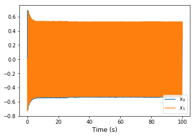
In the harmonic Oscillator example can anyone answer why the output experiences a ‘dampening’ at the start (in the first 5 seconds) and then becomes stable?
There is a lot to talk about here, as this is the interaction of a number of effects. But the really nice thing about Nengo is it lets us easily study these effects in isolation!
First of all, we can switch the neurons to “direct mode” by including neuron_type=nengo.Direct() in the call to nengo.Ensemble(..). This bypasses both neural representation (tuning curves) and spiking from the simulated ensemble, which allows us to focus purely on the intended macroscopic dynamics of the system.
# Create the model object
model = nengo.Network(label='Oscillator')
with model:
    # Create the ensemble for the oscillator
    neurons = nengo.Ensemble(200, dimensions=2, neuron_type=nengo.Direct())
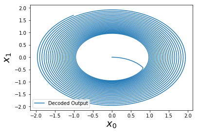
Curiously, the oscillation now expands outwards. If we were to run this further, we would see that it diverges off to infinity!
As it turns out, if we then reduce the time-step to dt=1e-4 (instead of the default of dt=1e-3), this problem seems to go away (or be reduced considerably).
# Create the simulator
with nengo.Simulator(model, dt=1e-4) as sim:
    ...
We have recently published a few papers (Voelker & Eliasmith, 2017 and Voelker & Eliasmith, 2018) that talk about this problem and the solution. The short story is that Principle 3 from the NEF does not account for the discrete nature of digital simulations. It assumes that the time-step is “sufficiently small” (i.e., approaching continuous time). However, this problem can be overcome by discretizing the desired dynamics and applying an extension of Principle 3 using the Z-transform in the discrete-time domain. This provides a procedure for implementing dynamical systems that behave identically even with different time-steps. This avoids the need to make dt smaller, which is costly from a simulation stand-point (it can be kept as is, or even be made larger).
For the example values of dt=1e-3 and synapse=0.1, we get (approximately):
transform=[[0.994975, 1.00499158], [-1.00499158, 0.994975]]
instead of the example’s transform=[[1, 1], [-1, 1]]. This matrix can be obtained numerically via the software package nengolib, and the analytical solutions are in the above papers (equations 21 and 4.7 for the first and second papers, respectively):
import nengolib
A, _, _, _ = nengolib.synapses.ss2sim(
    nengolib.signal.LinearSystem(([[0, 10], [-10, 0]], [[1], [0]], [[1, 0]], [[0]])),
    nengo.Lowpass(0.1), dt=0.001).ss
print(A)
(Note: The 10 comes from 1/0.1 for reasons related to the Principle 3 implementation in the example.)
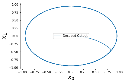
And now we have a perfect oscillator! It is perfect in the sense that it is equivalent to numerically solving the differential equations, up to some machine epsilon precision.
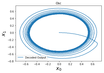
However… there is still something more going on. Switching gears back to neurons (removing Direct() mode), as you noticed, the example oscillator converged inwards to a steady limit cycle, instead of diverging outwards. The short explanation is that, since the decoders (the synaptic weights) are L2-regularized, the representation is biased towards under-approximating the output around the edge of the circle, thus pushing it inwards. I have a visualization of this at all points within the circle, as we modulate the direction of the oscillation:
These two competing forces — (1) inwards pressure from regularization, and (2) an outwards bias from the incorrect transform — happen to cancel out at the limit cycle that you observed.
We have seen already how to fix the second problem by changing the transform. We can limit the effect of the first problem by reducing the amount of L2-regularization, and increasing the number of neurons to improve the neural representation.
Yet, there is a third effect introduced by spiking. I won’t go into this right now since it’s material I need to unravel a bit more for my thesis, but you can see this by switching between neuron_type=nengo.LIF() and neuron_type=nengo.LIFRate(). An open challenge is to minimize the change in dynamics introduced by this latter switch!
As always, let me know if you have any follow-up questions and I can go into more detail.
Hi @arvoelke, the example above provides a really nice solution for using nengolib to generate the analytical solution to this system when using a lowpass synapse. However, I’m having some trouble accomplishing the same thing using a double exponential synapse: the system decays inward.
import numpy as np
import nengo
import nengolib
import matplotlib.pyplot as plt

dt = 1e-3
tauRise = 0.001
tauFall = 0.1
synapses = [nengolib.Lowpass(tauFall), nengolib.DoubleExp(tauRise, tauFall)]
labels = [f'Lowpass({tauFall})', f'DoubleExp({tauRise}, {tauFall})']

for i in range(len(synapses)):
	synapse = synapses[i]
	label = labels[i]
	A_ideal= [[0, 2*np.pi], [-2*np.pi, 0]]
	A_sim, _, _, _ = nengolib.synapses.ss2sim(
		nengolib.signal.LinearSystem(
			(A_ideal, [[1], [0]], [[1, 0]], [[0]])), synapse, dt=dt).ss
	print(A_sim)

	with nengo.Network() as model:
		kick = nengo.Node(lambda t: [tauFall/dt, 0] if t<=dt else [0,0])
		x = nengo.Ensemble(1, 2, neuron_type=nengo.Direct())
		nengo.Connection(kick, x, synapse=synapse)
		nengo.Connection(x, x, synapse=synapse, transform=A_sim)
		probe = nengo.Probe(x, synapse=None)

	with nengo.Simulator(model, dt=dt) as sim:
		sim.run(10)

	fig, ax = plt.subplots()
	ax.plot(sim.trange(), sim.data[probe], label=label)
	fig.savefig(f"{label}.pdf")
Lowpass(0.1).pdf (12.1 KB)
DoubleExp(0.001, 0.1).pdf (14.4 KB)
Am I missing something about the correct syntax for the ss2sim or LinearSystem functions?
Note that the inward decay is greatly reduced when using dt=1e-4.
Hey @psipeter. It’s been a while since I’ve looked into this but I believe this is explained in this comment block here:
A workaround is to build the double exponential synapse in such a way that the order of the numerator is zero after discretization. This can be done by discretizing each of the lowpass components and then multiplying them together (rather than multiplying them together before discretizing).
...
double_exp = (
    nengolib.signal.cont2discrete(nengo.Lowpass(tauRise), dt=dt) *
    nengolib.signal.cont2discrete(nengo.Lowpass(tauFall), dt=dt)
)
...
    dsys = nengolib.signal.cont2discrete(
        nengolib.signal.LinearSystem((A_ideal, [[1], [0]], [[1, 0]], [[0]])), dt=dt
    )
    A_sim, _, _, _ = nengolib.synapses.ss2sim(dsys, double_exp, dt=None).ss
That should give you the same oscillation now regardless of dt. There might be another more straightforward way to deal with this situation but it’s hard for me to know at the moment. @Eric was also looking at this recently in porting this over to Nengo core and could know something here.
That solves my issues with double exponential synapses and dt, thanks!