You are correct in the observation that for the specific objective function A^2 + B^2 + (A+B-0.5)^2, applying it naively to the PES rule will not work. This is because this specific function is always positive. Worse still, at the minima of the objective function, the value is non-zero. For other readers that want to know why this is an issue, I’ve explained it further down in this post.
In order to build a working system then, you’ll need to reframe the PES error value such that it has a positive and negative value, depending on which way you need the decoders to be adjusted. For this objective function in particular, the gradients (partial derivatives) of each variable in the objective function can be used to provide such a signal. The gradient is particularly useful in this scenario because the objective function is at a minimal value when the derivative of it is 0. Additionally, the gradients have the right sign, where a negative gradient should drive up a value, and a positive gradient should drive down a value.
For your particular problem, using the gradient as the PES error signal is straightforward. Changes to the value of A should be driven by \frac{\partial f}{\partial A}, and changes to the value of B should be driven by \frac{\partial f}{\partial B}. You can implement this in Nengo multiple ways, either with one ensemble each representing A and B, or you can have one 2D ensemble representing both A and B. Other than that, all you need to do is to compute the partial derivatives, and use the result as the learning rule error signal. If you have two ensembles for A and B, you’ll need two connections and two error signals. If you used one ensemble, you can combine both partial derivatives into one 2D error signal. In the code snippet below, I’ve used an ensemble each for A and B.
import nengo

def part_A_func(x):
    return 4 * x[0] + 2 * x[1] - 1

def part_B_func(x):
    return 4 * x[1] + 2 * x[0] - 1

with nengo.Network() as model:
    ensA = nengo.Ensemble(50, 1)
    ensB = nengo.Ensemble(50, 1)
    out = nengo.Ensemble(100, dimensions=2)

    conn1 = nengo.Connection(ensA, out[0])
    conn1.learning_rule_type = nengo.PES()
    conn2 = nengo.Connection(ensB, out[1])
    conn2.learning_rule_type = nengo.PES()

    nengo.Connection(out, conn1.learning_rule, function=part_A_func, synapse=0.1)
    nengo.Connection(out, conn2.learning_rule, function=part_B_func, synapse=0.1)

    part = nengo.Node(size_in=2)
    nengo.Connection(out, part[0], function=part_A_func, synapse=0.1)
    nengo.Connection(out, part[1], function=part_B_func, synapse=0.1)

    p_out = nengo.Probe(out, synapse=0.1)
    p_part = nengo.Probe(part)

with nengo.Simulator(model) as sim:
    sim.run(10)
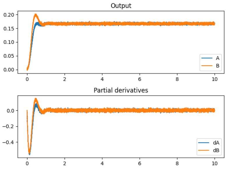
If we run this code, we get a plot like so:
And from this plot, we can see that the system does converge to approximately the correct values – according to Wolfram Alpha, the objective function is minimized when A=1/6 and B=1/6.
Now, this approach may not always work, and is dependent on the objective function used. Regardless, the key takeaway from this exercise is that to get around the limitations of the objective function (i.e., it never going negative), one needed to reframe the problem and find a way to generate error signals that could be used with the PES learning rule.
Side note: Why an always-positive error signal is bad for the PES
The PES learning rule works by modifying the decoders of a Nengo connection in the direction opposite of the error signal. I.e., if the error signal is positive, the decoded output of the learned population will be driven in the negative direction (and vice versa for a negative error value). This behaviour poses an issue if the function used to calculate the error signal is always positive for the range of values it is trying to optimize over.
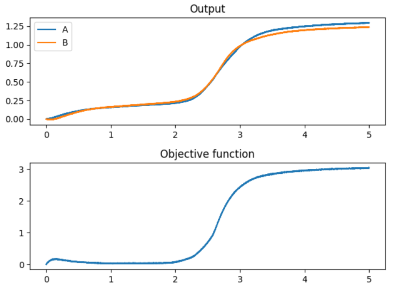
Take the objective function above (A^2 + B^2 + (A+B-0.5)^2) as an example. If we were to use the negative output of the objective function as the input to the “error” signal of the PES learning rule, it would initially do as expected. That is to say, it would increase the represented values of A and B in order to reduce the error value, as demonstrated by this plot:
However, once the objective function reaches it’s minimum value (when the objective function is equal to 1/12), it is still positive, which means that rather than the PES learning rule stopping (ideally it should stop when the minima is reached), the PES error would continue to increase the values of A and B in an attempt to continue decreasing the output of the objective function. However, this just works to increase the output of the objective function, which creates a positive feedback loop, forever increasing the values of A and B: