Neural implementation of Arctangent2

[MatthijsPals]

Hey all,

I am running in some problems with a nengo implementation of a model executing a delayed-response task. I have two ensembles (lets call them A and B) that both represent an orientation. Ensemble A represents the orientation by means of sine and cosine of theta. Ensemble B represents the orientation by means of sine and cosine of theta multiplied by some unkown constant a that varies with time.

So we have the following:

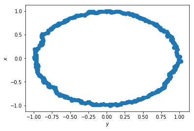
ensemble A represents: sine(theta), cosine(theta)
ensemble B represents: a sine (theta), a cosine(theta)

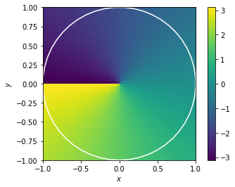
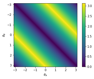
I need to decode the difference between theta represented in ensemble A and B, For this I could simply use the arctan2 function:

diff_thetaAB= arctan2(sinA, cosA)-arctan2(sinB, cosB)

which should also gets rid of the unkown mupltiplier a as arctan2(sin, cos) equals arctan2(a sin, a cos)

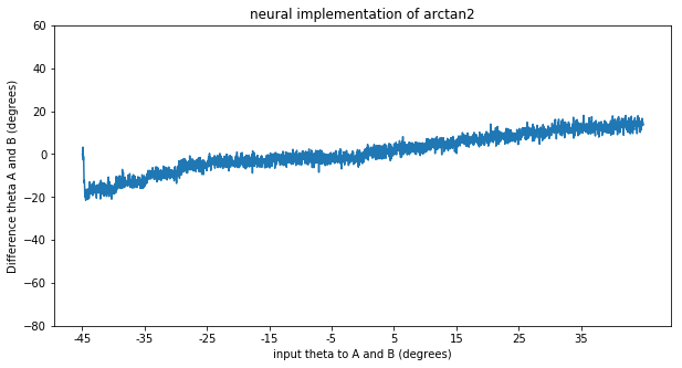
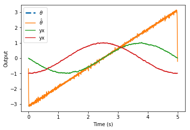
This all works fine if I use a non-neural implementation of arctan2 (by setting the neuron_type to nengo.Direct()). However as soon as I calculate the arctan2 function with spiking neurons I start to run into problems. I’ve added a simple model that just highlights the problem below. The neurons do quite a bad job of approximating the arctan2 function (which might be expected as its shape is not continuous). However they don’t just compute a noisy version of arctan2, they are consistently worse for some theta as shown in the second graph below.

The model I used to create the graph has two ensembles A and B that are both fed the same orientation, with a set to 0.1. The input goes from theta -45 to theta is 45 degrees in steps of 5 degrees every 0.25 seconds as noted on the x axis. The y-axis represents the difference in theta decoded from the sine and cosine of ensemble A and B. First with a neural implementation and secondly with a direct implementation.

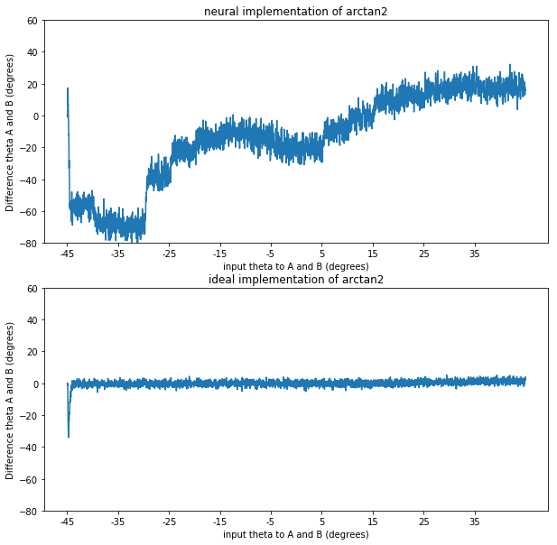
As seen in the direct implementation we would expect a difference of 0, as both ensemble A and B are fed the same orientation. However the neural implementation consistently gives a “negative” difference for a negative orientation and a “positive” difference for a positive input orientation as can be seen in the graph. (It wouldn’t be problematic for my model if the neurons just did a noisy implementation, but that is clearly not the case)

So my question is, why is there this consistent error in the neural implementation of the arctan2 function? Does this have something to do with the shape of the function? If so, is it possible to implement it in such a way that gets rid of this problem? (by optimizing it just over the range for which it is continuous maybe?) Or is there another way I could decode the orientation difference theta represented in two ensembles from their sine and cosine of theta?

Please let me know if you have any questions. I would be very grateful if anybody can help me shed some light on this problem!

[MatthijsPals]

This is the model used to create the graph shown above

import numpy as np
import matplotlib.pyplot as plt   
import nengo
import math
from stp_ocl_implementation import *
import pyopencl as cl

#input to the network, varying values of theta
theta=np.arange(-45,45,5)/180*math.pi
sin=np.sin(theta)
cos=np.cos(theta)

def input_func(t):
    i=math.floor(t/0.25)
    return np.sin(theta[i]),np.cos(theta[i])

#calculate difference between theta of A and B via their sine and cosine
def arctan_func(v):
    x1,y1,x2,y2=v
    return np.arctan2(x1,y1)-np.arctan2(x2,y2)

with nengo.Network() as model:
        
    #ensemble A and B both represent the sine and cosine of theta
    input_Node=nengo.Node(input_func)     

    ensemble_A = nengo.Ensemble(1000, dimensions=2)
    ensemble_B = nengo.Ensemble(1000, dimensions=2)
        
    nengo.Connection(input_Node, ensemble_A)
    nengo.Connection(ensemble_A, ensemble_B,transform=.1)
    
    #arctan calculates the difference between the theta represented by ensemble A and B
    arctan = nengo.Ensemble(1000, dimensions=4, radius=1)
    out = nengo.Ensemble(500, dimensions=1, radius=math.pi)
    
    nengo.Connection(ensemble_A, arctan[:2])
    nengo.Connection(ensemble_B, arctan[2:])
    nengo.Connection(arctan, out, function=arctan_func)
    
    #a nengo.Direct() implementation for comparison
    arctan_direct = nengo.Ensemble(1000, dimensions=4, neuron_type=nengo.Direct())
    out_direct = nengo.Ensemble(500, dimensions=1, radius=math.pi)
    
    nengo.Connection(ensemble_A, arctan_direct[:2])
    nengo.Connection(ensemble_B, arctan_direct[2:])
    nengo.Connection(arctan_direct, out_direct, function=arctan_func)  
    
    #probes
    p_out=nengo.Probe(out, synapse=0.01)
    p_out_direct=nengo.Probe(out_direct, synapse=0.01)

[MatthijsPals]

A big improvement seems to be made when only optimizing arctan over a part where it is continuous, as follows (if I understand this correctly):

#create space to optimize over (creating this randomly is probably not the most efficient)
N=10000                          #amount of samples
Sin1=2*np.random.random(N)-1     #arctan is continuous when sin is between -1 and 1
Cos1=np.random.random(N)         #and cos vis between 0 and 1
Sin2=2*np.random.random(N)-1
Cos2=np.random.random(N)
ep=np.transpose(np.vstack((Sin1,Cos1,Sin2,Cos2)))  #eval points

answers=np.transpose([np.arctan2(ep[:,0],ep[:,1])-np.arctan2(ep[:,2],ep[:,3])])  #orientation difference for those eval points

#optimize arctan only over continuous part
nengo.Connection(arctan, out, eval_points=ep, function=answers)

However for values of a smaller than 1 (ensemble B represents a sine (theta), a cosine(theta)), we still have the same skew.

Edit: I do wonder if this argument of optimizing over a continuous surface still holds when the input is 4d (arctan(a,b)-arctan(c,d)) instead of 2d (arctan(a,b))

[arvoelke]

Welcome @MatthijsPals! Thanks for posting some code and showing what you have tried. That definitely helps!

Indeed most of the difficulty in this function stems from the discontinuity in arctan2(y, x) (note that the first argument to np.arctan2 is $y$ and the second argument is $x$). Visualizing this as a surface (credit to @tcstewar for the suggestion):

W = np.linspace(-1, 1)
X, Y = np.meshgrid(W, W)
Z = np.arctan2(Y, X)
theta = np.pi*W

plt.figure()
plt.plot(np.cos(theta), np.sin(theta), c='white')
plt.xlabel("$x$")
plt.ylabel("$y$")
plt.imshow(Z, extent=[-1, 1, -1, 1])
plt.colorbar()
plt.show()

We see that there is a sudden cliff from $+\pi$ to $-\pi$ right around where $y$ crosses over $0$ (for $x < 0$).

It is important to keep in mind that you are attempting to fit the entire surface within the unit circle $x^2 + y^2 \le 1$ by weighting together tuning curves that are continous in space. Mathematically there is no way to achieve a perfect discontinuity in your output space by weighting together basis functions that are continuous. As a result, the decoders will try their best to compensate around these end-points with some L2-regularization, resulting in the skew that you have observed.

We can do a little better by restricting the eval_points as you suggested above, but there is still a discontinuity at $x = -1$ and $y = 0$. This suggests to me either that:

1. This is unlikely to be a space that neurons represent. It could be better to use some alternate representation (e.g., polar-coordinates), or restrict your $(x, y)$ to some continuous subspace.

2. Neurons that could potentially implement this spatial discontinuity would require a discontinuity in their response curves. For example, an increasing amount of current would need to suddenly shut the neuron off.

For fun, I’ve thrown together a quick demonstration of how a “sawtooth ReLU” in rate-mode can approximate the discontinuous part of the surface a little bit better than a continuous neuron. This can very likely be improved by being more clever about the arrangement of tuning curves.

import numpy as np
import nengo
import matplotlib.pyplot as plt

class LinearSawtooth(nengo.RectifiedLinear):
    """RectifiedLinear with wraparound."""
    
    output_threshold = nengo.params.NumberParam(
        'output_threshold', low=0, low_open=True)

    def __init__(self, output_threshold=100.0, *args, **kwargs):
        super().__init__(*args, **kwargs)
        self.output_threshold = output_threshold

    def step_math(self, dt, J, output):
        super().step_math(dt, J, output)
        output %= self.output_threshold

sim_t = 5.0
tau_probe = None
neuron_type = LinearSawtooth()

with nengo.Network(seed=0) as model:
    
    theta = nengo.Node(output=lambda t: np.pi*(2*t/sim_t - 1))

    yx = nengo.Ensemble(2500, 2, neuron_type=neuron_type)
    
    nengo.Connection(
        theta, yx[0], function=lambda theta: np.sin(theta), synapse=None)
    nengo.Connection(
        theta, yx[1], function=lambda theta: np.cos(theta), synapse=None)
    
    theta_hat = nengo.Node(size_in=1)
    
    nengo.Connection(
        yx, theta_hat, function=lambda yx: np.arctan2(*yx), synapse=None,
        eval_points=nengo.dists.UniformHypersphere(surface=True),
    )
    
    p_theta = nengo.Probe(theta, synapse=tau_probe)
    p_yx = nengo.Probe(yx, synapse=tau_probe)
    p_theta_hat = nengo.Probe(theta_hat, synapse=tau_probe)

with nengo.Simulator(model) as sim:
    sim.run(sim_t)

plt.figure()
plt.plot(sim.trange(), sim.data[p_theta],
         label=r"$\theta$", linestyle='--', lw=3)
plt.plot(sim.trange(), sim.data[p_theta_hat],
         label=r"$\hat{\theta}$")
plt.plot(sim.trange(), sim.data[p_yx], label="yx")
plt.xlabel("Time (s)")
plt.ylabel("Output")
plt.legend()
plt.show()

plt.figure()
plt.scatter(*sim.data[p_yx].T)
plt.xlabel("$y$")
plt.ylabel("$x$")
plt.show()

[MatthijsPals]

Thank you a lot! The plots definitely help clearing things up.

This is unlikely to be a space that neurons represent. It could be better to use some alternate representation (e.g., polar-coordinates), or restrict your (x,y)(x,y) to some continuous subspace.

Polar-coordinates wouldn’t work in this case I think, since the second ensemble in my network would then represent a(r, θ), where a is an unkown constant, losing the correct angle. (which we retain if we represent a sin(θ), a cos (θ) ).

Optimizing over a subspace might then be the best option. The maximum orientation difference between stimuli in the experiment I am trying to model is 42 degrees, so the model should be able to function properly when just using a continuous subspace (although it might lose in plausibility).

I still have two questions. First, do we find something like sawtooth tuning curves for actual neurons?

Second, I am a bit confused about the continuity of a 4d input space. Say I have a connection that computes:

out = arctan2(y1, x1) - arctan2(y2, x2)

would the input space be continuous if I keep y1 and y2 between 0 and 1 and x1 and x2 between -1 and 1? Or does this simply not hold for multidimensional space? (in which cases I might be able delegate the computation of both arctans do different ensembles and then substract them)

Thank you so much!

[arvoelke]

To clarify the task, the two thetas represented by each population can differ by up to 42 degrees, and $a$ is the (time-varying) length of the second vector? So in polar coordiantes (length, angle) we have $(1, \theta_A)$ for ensemble A and $(a, \theta_B)$ for ensemble B, and the task is to output the (absolute?) difference between the two angles?

Polar-coordinates wouldn’t work in this case I think, since the second ensemble in my network would then represent a(r, θ) , where a is an unkown constant, losing the correct angle. (which we retain if we represent a sin(θ), a cos (θ) ).

The benefit of polar coordiantes is the angles are directly a part of the representation. If you were to start with a polar coordinate representation, then I think a solution would be to output $\theta_A - \theta_B$ with some special handling of the various ways that $\theta$ can wrap-around $\pm \pi$ (otherwise you would have $+\pi$ being very far away from $-\pi$ when in fact they are the same angle):

W = np.linspace(-np.pi, np.pi, 1000)
thA, thB = np.meshgrid(W, W)
Z = np.min([np.abs(thA - thB),
            np.abs(thA - thB + 2*np.pi),
            np.abs(thA - thB - 2*np.pi)], axis=0)

plt.figure()
plt.xlabel(r"$\theta_A$")
plt.ylabel(r"$\theta_B$")
plt.imshow(Z, extent=[-np.pi, np.pi, np.pi, -np.pi])
plt.colorbar()
plt.show()

This surface would be much easier for neurons to compute.

That said… it seems to me the difficulty in the 4D case is really coming from the fact that you aren’t handling the boundary cases of $\theta$ wrapping around $\pm \pi$ in the above way. Currently if you have two points, one with $\theta_A = \pi$ and the other with $\theta_B = -\pi$, then the answer should be close to zero, and not $\pm 2\pi$. If you handle these cases correctly then the discontinuities from each of the two np.arctan2 functions should actually cancel out!

Could you try the function:

def angle_diff(xA, xB, yA, yB):
    z = np.arctan2(yA, xA) - np.arctan2(yB, xB)
    return np.min([np.abs(z),
                   np.abs(z + 2*np.pi),
                   np.abs(z - 2*np.pi)])

and see if that helps?

To see why this should help, we can consider an alternate way of deriving this exact same function that does not use np.arctan2. Starting with:
$$\begin{align}(x_A, y_A) &= (\cos(\theta_A), \sin(\theta_A)) \\ (x_B, y_B) &= (a \cos(\theta_B), a \sin(\theta_B))\end{align}$$
we can draw a triangle between the points $(0, 0)$, $(x_A, y_A)$, and $(x_B, y_B)$. The desired output corresponds to the interior angle of the triangle at point $(0, 0)$.

The law of cosines provides a formula for finding the angle of a triangle given its side-lengths. We know the side from the origin to $A$ has length $1$, the side from the origin to $B$ has length $a = \sqrt{x_B^2 + y_B^2}$, and the remaining side from $A$ to $B$ has length $\sqrt{\left(x_A - x_B\right)^2 + \left(y_A - y_B\right)^2}$. Plugging this into the law of cosines and rearranging gives:

$$\arccos \left[ \frac{\left(x_A - x_B\right)^2 + \left(y_A - y_B\right)^2 - 1 - \left(x_B^2 + y_B^2\right) }{ - 2 \sqrt{x_B^2 + y_B^2} } \right] $$

The key observation is that this is differentiable with respect to $(x_A, x_B, y_A, y_B)$ assuming that $a > 0$. In other words, as long as your second vector has some non-zero length, this 4D function is actually continuous.

Here is a quick sanity check that the two functions are the same:

def angle_diff_v2(xA, xB, yA, yB):
    asq = xB**2 + yB**2
    return np.arccos(((xA - xB)**2 + (yA - yB)**2 - 1 - asq) /
                     (-2 * np.sqrt(asq)))

thA = np.pi/4
thB = -0.1
a = 0.6

xA = np.cos(thA)
yA = np.sin(thA)
xB = a*np.cos(thB)
yB = a*np.sin(thB)

print(angle_diff(xA, xB, yA, yB))
print(angle_diff_v2(xA, xB, yA, yB))

0.8853981633974483
0.885398163397448

First, do we find something like sawtooth tuning curves for actual neurons?

That was just me having fun to make a point about how the kinds of functions that neurons can compute are coupled to the shapes of their response curves. Eliasmith and Anderson (2003) has a chapter that analyzes this using SVD for LIF neurons and cosine tuning and finds they are good at polynomial functions and the Fourier basis, respectively.

Second, I am a bit confused about the continuity of a 4d input space.

I hope I managed to answer this in a round-about way. To summarize the individual 2D np.arctan2 functions are themselves discontinuous, but when you subtract them and handle the various ways that the angles can wrap around $\pm \pi$, then the overall function in fact becomes continuous! Therefore, it is probably best to do this function in one step using either of the two forms I gave above.

[MatthijsPals]

To clarify the task, the two thetas represented by each population can differ by up to 42 degrees

Yes! And then in the end the network is to indicate whether the orientation in ensemble A is turned left or right with respect to the orientation in ensemble B (by using the orientation difference between the two)

To clarify the task, the two thetas represented by each population can differ by up to 42 degrees, and $a$ is the (time-varying) length of the second vector? So in polar coordiantes (length, angle) we have $(1, \theta_A)$ for ensemble A and $(a, \theta_B)$ for ensemble B, and the task is to output the (absolute?) difference between the two angles?

Anything ensemble B represents will be multiplied by the time-varying $a$ (due to how the memory system is implemented). Thus in this case I don’t think it would be possible to represent $(a, \theta_B)$, because $(a, a*\theta_B)$ would be represented instead. Indeed the network should output the difference between the two angles. However we should not use the absolute difference, as we need the sign in order to say whether one orientation is turned left or right with respect to the other.

Could you try the function and see if that helps?

I tried creating a variant of the function in your post that outputs the signed difference:

def arctan_func(v):
    yA, xA, yB, xB=v
    z = np.arctan2(yA, xA) - np.arctan2(yB, xB)
    pos_ans = [z, z+2*np.pi, z-2*np.pi]
    i = np.argmin(np.abs(pos_ans))
    return pos_ans[i]

At first sight this seems to work really well! I will now try to run a larger number of trials with my full model and report back.

By the way, I would not be able to use the arccos variant right? As the range of arccos is $[0, \pi]$, we lose the sign.

Thank you so much for your insight and taking the time to answer my questions!

[arvoelke]

Oh I see. And nice approach to getting the signed difference. That looks to me like the right thing to be doing then.

Good point about arccos only giving half the range. There might be a way to extend the approach from my last post to get the sign right as well, but since all that matters is the input-output behaviour of this function (i.e., target points for the decoders to fit, with respect to the sampled eval_points) what you have here should be good!

Let us know if the model is still struggling to perform and we can look into some other possibilities for improvement.

[arvoelke]

A quick note though: when switching from the abs difference to the signed difference, this lost continuity. An intuitive way to see why is because the function $f(x) = |x|$ wraps around the domain $x \in [-1, 1]$, while the function $f(x) = x$ does not (there is a discontinuity at $x = \pm 1$).

In the context of the 4D function, a counter-example is:

def arctan_func(v):
    yA, xA, yB, xB=v
    z = np.arctan2(yA, xA) - np.arctan2(yB, xB)
    pos_ans = [z, z+2*np.pi, z-2*np.pi]
    i = np.argmin(np.abs(pos_ans))
    return pos_ans[i]

def g(thA, thB, a):
    xA = np.cos(thA)
    yA = np.sin(thA)
    xB = a*np.cos(thB)
    yB = a*np.sin(thB)
    return arctan_func([yA, xA, yB, xB])

print(g(0, -np.pi, 1))
print(g(0, +np.pi, 1))

3.141592653589793
-3.141592653589793

I believe this discontinuity only happens when the difference between the angles is $\pm \pi$. Since you said in your experiment it’s at most $\pm 42$ degrees, this should not be an issue except when choosing the 4D evaluation points to sample. By letting Nengo pick points near the discontinuity, it might be making the approximation worse than it could potentially be. It might be better to forward-generate a bunch of eval_points by generating a random angle between $[-42, 42]$ degrees, a random 2D vector from the surface of the hypersphere, and a random scaling factor (preferably not too close to zero), and then using that to construct the 4D evaluation point (and repeating a couple thousand times). Also make sure the radius of this ensemble is set appropriately. Good luck!

[MatthijsPals]

Thanks! Good point about the lost continuity when keeping the sign, I didn’t realise that.

It might be better to forward-generate a bunch of eval_points by generating a random angle between $[-42, 42]$ degrees, a random 2D vector from the surface of the hypersphere, and a random scaling factor (preferably not too close to zero), and then using that to construct the 4D evaluation point (and repeating a couple thousand times).

Would I do that as follows or is there a smarter way?

#amount of samples
N=10000

#generate random initial orientation A using Hypersphere
sinAcosA=nengo.dists.UniformHypersphere(surface=True).sample(N,2)
thetaA=np.arctan2(sinAcosA[:,0],sinAcosA[:,1])

#angle difference between A and B of max 42 degrees
thetaDiff=(84*np.random.random(N)-42)/180*np.pi

#calculate corresponding orientation B 
thetaB=thetaA+thetaDiff
sinBcosB=np.vstack((np.sin(thetaB),np.cos(thetaB)))

#scale with factor beteen 0.1 and 1
scale=np.random.random(N)*0.9+0.1
sinBcosB=sinBcosB*scale

#generate evalpoints
ep=np.vstack((sinAcosA.T,sinBcosB))

Also make sure the radius of this ensemble is set appropriately.

Would the ensemble that computes the arctan need a radius larger than 1? Or just the recieving ensemble, which needs a radius of 42 if the output is in degrees.

[arvoelke]

I didn’t review too carefully but looks right and can’t think of a clever way off-hand to shorten that. You’ll need to transpose ep though to have the shape (N, 4). As a sanity check it might help to plot a few evaluation points (e.g., two points per scatter plot) and see if the output of your function makes sense for each pair.

Would the ensemble that computes the arctan need a radius larger than 1? Or just the recieving ensemble, which needs a radius of 42 if the output is in degrees.

The radius is always with respect to the vectors being represented by the ensemble, and so the post ensemble would need to be 42 if you have a transform that is converting to degrees. The ensemble that computes the arctan would need a radius of $\sqrt{2}$ since the largest 4D vector has a length of $\sqrt{(1^2 + 0^2) + (1^2 + 0^2)}$ (as an example). Any nengo.Connection you make from this pre ensemble need to set scale_eval_points=False otherwise the eval_points that you pass in will be scaled by the same $\sqrt{2}$ factor. The reason this scaling is on by default is because usually you would want to have the interior of the unit hypersphere scaled by the radius, but here you’re no longer optimizing over that same space. Hope this makes sense.

[MatthijsPals]

Thanks a lot again, the model seems to performing well now!

The ensemble that computes the arctan would need a radius of $\sqrt{2}$ since the largest 4D vector has a length of $\sqrt{(1^2 + 0^2) + (1^2 + 0^2)}$ (as an example).

I guess I am still a little bit confused about why the radius needs to be set to the largest possible length of the vector, and not just to the largest possible value of its elements. If I understood correctly the radius is used to determine the range of the elements of a vector an ensemble represents. Is the representation not optimized for $[-radius, radius]$ for each element of the to-be-represented vector seperately?

Any nengo.Connection you make from this pre ensemble need to set scale_eval_points=False otherwise the eval_points that you pass in will be scaled by the same $\sqrt{2}$ factor. The reason this scaling is on by default is because usually you would want to have the interior of the unit hypersphere scaled by the radius, but here you’re no longer optimizing over that same space. Hope this makes sense.

Thanks, I wasn’t aware of that option, but that makes sense!

[arvoelke]

I guess I am still a little bit confused about why the radius needs to be set to the largest possible length of the vector, and not just to the largest possible value of its elements. If I understood correctly the radius is used to determine the range of the elements of a vector an ensemble represents. Is the representation not optimized for [−radius,radius][−radius,radius][-radius, radius] for each element of the to-be-represented vector seperately?

Good question. Each neuron’s “encoder” is, by default, normalized to the surface of the unit hypersphere and scaled inversely by the ensemble’s radius (this happens to be convenient for a number of reasons). If you were to set the radius to 1 then let’s suppose one of the encoders ends up being $e = (1/\sqrt{2}, 0, 1/\sqrt{2}, 0)$ which is on the surface of the unit hypersphere ($||e|| = 1$). Next consider the input vector $x = (1, 0, 1, 0)$. The neuron’s input current ends up being (a scaled and shifted version of) dot(e, x) = sqrt(2) which is outside the unit range that the neuron’s response curve is distributed across. What this means is that some of your neurons might begin to “saturate” near the maximum firing-rates and possibly produce activities that weren’t accounted for during decoder optimization (this depends on chosen evaluation points). Often this can be somewhat innocuous if not too far outside the radius, but in general this will impact the accuracy for certain inputs.

However if you pick a radius of sqrt(2) then that same encoder would end up being $e = (1/2, 0, 1/2, 0)$ in which case dot(e, x) = 1 which is okay. Basically, here you want to pick the radius in a way that scales the hypersphere to encompass the domain of x, which you can do by setting it to the maximum length.

That said this is not a strict requirement or limitation, much like everything else in Nengo. Helper networks such as nengo.networks.EnsembleArray represent each dimension independently and thus a radius of 1 would be perfectly okay in this case. Similarly, you can consider distributions that allow for encoders to be on the corners of the “hypercube” and then set normalize_encoders=False on the Ensemble to prevent them from being renormalized. The defaults are intended to capture the majority of typical use cases, but all of this is highly configurable.

[MatthijsPals]

Thank you for clearing that up as well. Turns out I had to account for this in the input ensemble of my model as well, the resulting signal is a lot less noisy now!