Nengo summer school 2020 - Basic integrator memory vs State memory

Hi,
I’ve got question about 6th lecture. Chris or Terry showed us a “State” component from SPA, as a multidimensional integrator example.
I think that “State” object, with feedback=1 isn’t just an integrator, as shown in previous examples. If I feed some value (1 or more D vector) into a standard integrator, it will saturate over time. In the case of a “State” component, you can feed in any value, and it will not saturate ever, rather roughly stick to that value. Could you explain that and how does this component work?

Thank you very much for whole Nengo summer school videos and for the explanation :slight_smile:

Hello @FilipD, and thank you for the most interesting question!

I must admit, I was quite stumped with this question myself. Initially, I had thought that the answer was simple: The saturation dynamics of an integrator in a higher dimensional space are different than that of a 1D integrator. As it turns out, my intuition about integrator dynamics was completely wrong (and it took some experimentation to figure this out), and this isn’t the actual answer, as I will demonstrate below.

First, to the claim that feeding in a regular-ol’ integrator would cause the output to saturate over time. I presume you mean that the output would “saturate” at a value above that of 1. From my experimentation, this is actually not the case. The code below creates two Nengo ensembles, both with the same neuron parameters. One ensemble is set up as a integrator, and the other is left in the feedforward configuration. The input to the integrator is a constant input of 1. The input to the “feed-forward” ensemble is a ramp that emulates the ramp output of an ideal (non-neural) integrator. Both ensembles use the LIFRate neuron type for smoother plots, but the findings generalize to spiking neurons as well.

Here’s the code:

import time
import nengo
import matplotlib.pyplot as plt


with nengo.Network() as model:
    neuron_type = nengo.LIFRate()
    nn = 50
    radius = 1

    seed = int(time.time())
    print("Using seed: ", seed)

    ramp_scale = 1
    ramp = nengo.Node(lambda t: t * ramp_scale)
    level = nengo.Node(ramp_scale)

    ens_ens = nengo.Ensemble(nn, 1, seed=seed, neuron_type=neuron_type, radius=radius)
    nengo.Connection(ramp, ens_ens)

    tau = 0.1  # Feedback synapse for the integrator
    int_ens = nengo.Ensemble(nn, 1, seed=seed, neuron_type=neuron_type, radius=radius)
    nengo.Connection(level, int_ens, transform=tau, synapse=tau)
    nengo.Connection(int_ens, int_ens, synapse=tau)

    p_ramp = nengo.Probe(ramp)
    p_ens = nengo.Probe(ens_ens, synapse=0.01)
    p_int = nengo.Probe(int_ens, synapse=0.01)

with nengo.Simulator(model) as sim:
    sim.run(3)


plt.figure()
plt.plot(sim.trange(), sim.data[p_ens], label="ens")
plt.plot(sim.trange(), sim.data[p_int], label="integrator")
plt.plot(sim.trange(), sim.data[p_ramp], 'k--', label="ramp")
plt.plot([0, 3], [radius, radius], 'r--')
plt.ylim(0, 2)
plt.legend()
plt.show()

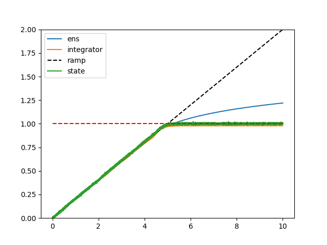
And here is the resulting plot!
image

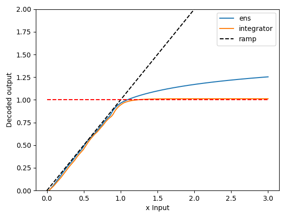
Let’s take a closer look at the plot, and make some observations:

  1. The output of the integrator and feed-forward ensemble both follow the ideal ramping behaviour quite closely. This means that the integrator is doing what it is meant to do (integrate a constant input to output a ramp), and so is the feed-forward ensemble (take the ramp into and output a ramp output).
  2. From $x=0$ to $x=1$, the feed-forward output follows the integrator output quite closely. We would expect this to be the case since both ensembles have been initialized with the same neuron parameters. It’s not 100% identical because the feed-forward ensemble doesn’t account for the feedback dynamics present in the integrator ensemble.
  3. Past $x=1$, the output of the feed-forward ensemble isn’t able to stick to the ramp ideal, but, this is to be expected as the ensemble is optimized in the range of $-1 < x < 1$, so everything outside that range is off the table.
  4. Also, as expected, when the feed-forward ensemble is driven with a large enough input, the output of the ensemble saturates (doesn’t keep increasing) because the neurons themselves are firing at their maximum rates.
  5. The output of the integrator “saturates” at about 1! Honestly, when I first saw this, I double checked my code thinking I had made a mistake. My original intuition was the saturation behaviour should reflect that of the feed-forward ensemble (which is clearly not the case here).

So… what is going on here? Why does the output of the integrator “saturate” at about 1? The output of the feed-forward ensemble in the plot above gives us a clue. You can think about an integrator as a bunch of fixed points, with the input to the integrator acting to push the value stored in the integrator from fixed point to fixed point. In an ideal integrator, the fixed points are infinitely close together. However, in the neural integrator, the fixed points are determined by crossing points where the neural output crosses the $y=x$ line. Coincidentally, the $y=x$ line is also the ramp input we provided to the feed-forward ensemble, so we can look at that output to deduce the behaviour of the integrator. And, if you look at the output, you’ll notice that about $x=0.92$, the output of the neural ensemble starts to diverge from the ideal $y=x$ line. What this means is that for any input greater than $x=0.92$, the integrator’s feedback value will be less than the input, stopping the integrator from integrating any further, and the value of the integrator falls back to the last fixed point (plus the input value) – which happens (for this seed) to be about 1 (0.92 + 0.1 [the input] ~= 1.02 [the observed value]). If you run the code multiple times, you’ll see that the “saturation” value of the integrator varies from run to run, sometimes below 1, sometimes above 1, but generally about 1.

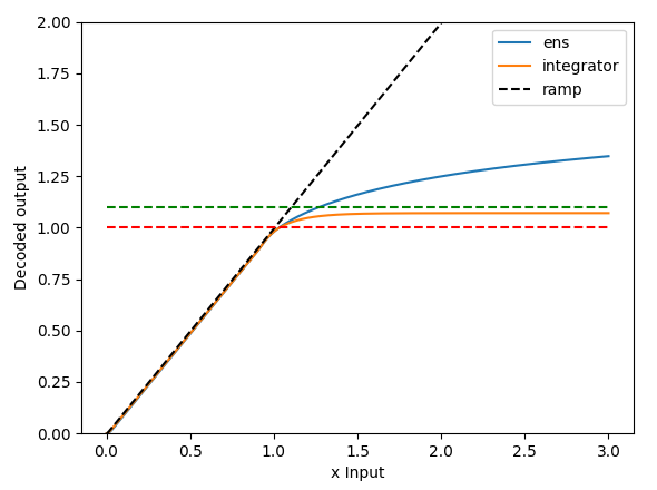
And you can experiment with the code as well. By increasing the number of neurons in the integrator to some super large number (the plot below uses 10000), the integrator becomes more ideal, so the last fixed point approaches $x=1, y=1$. In the graph below, the last fixed point is about 0.98, so with the input of about 0.1, the “saturated” integrator value is about 1.08 (the green dashed line represents 1.1)

image

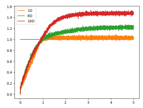
Okay. So that’s the integrator “saturation” behaviour in 1 dimension. What about multiple dimensions? Well, this behaviour extends to multiple dimensions as well (which answers your original question).

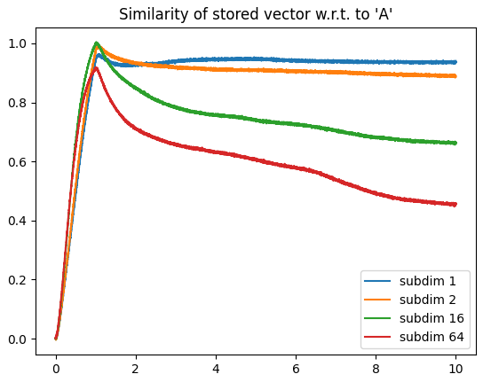
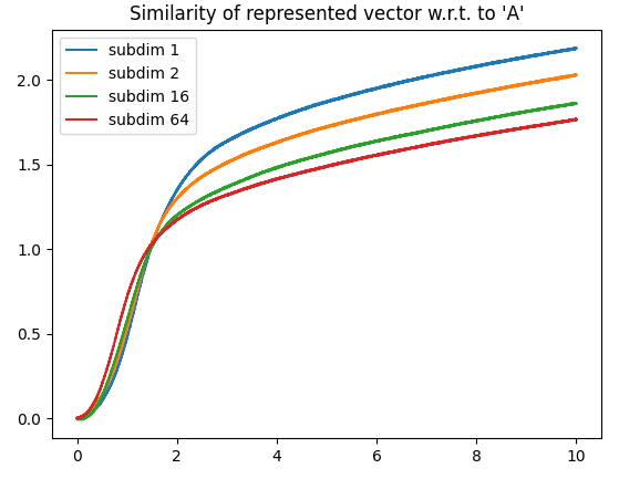
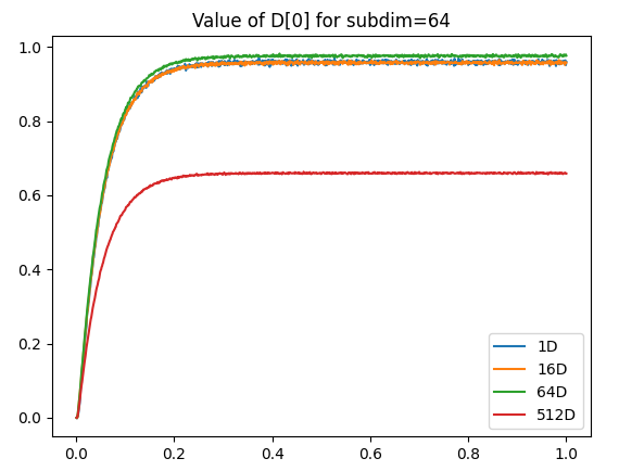
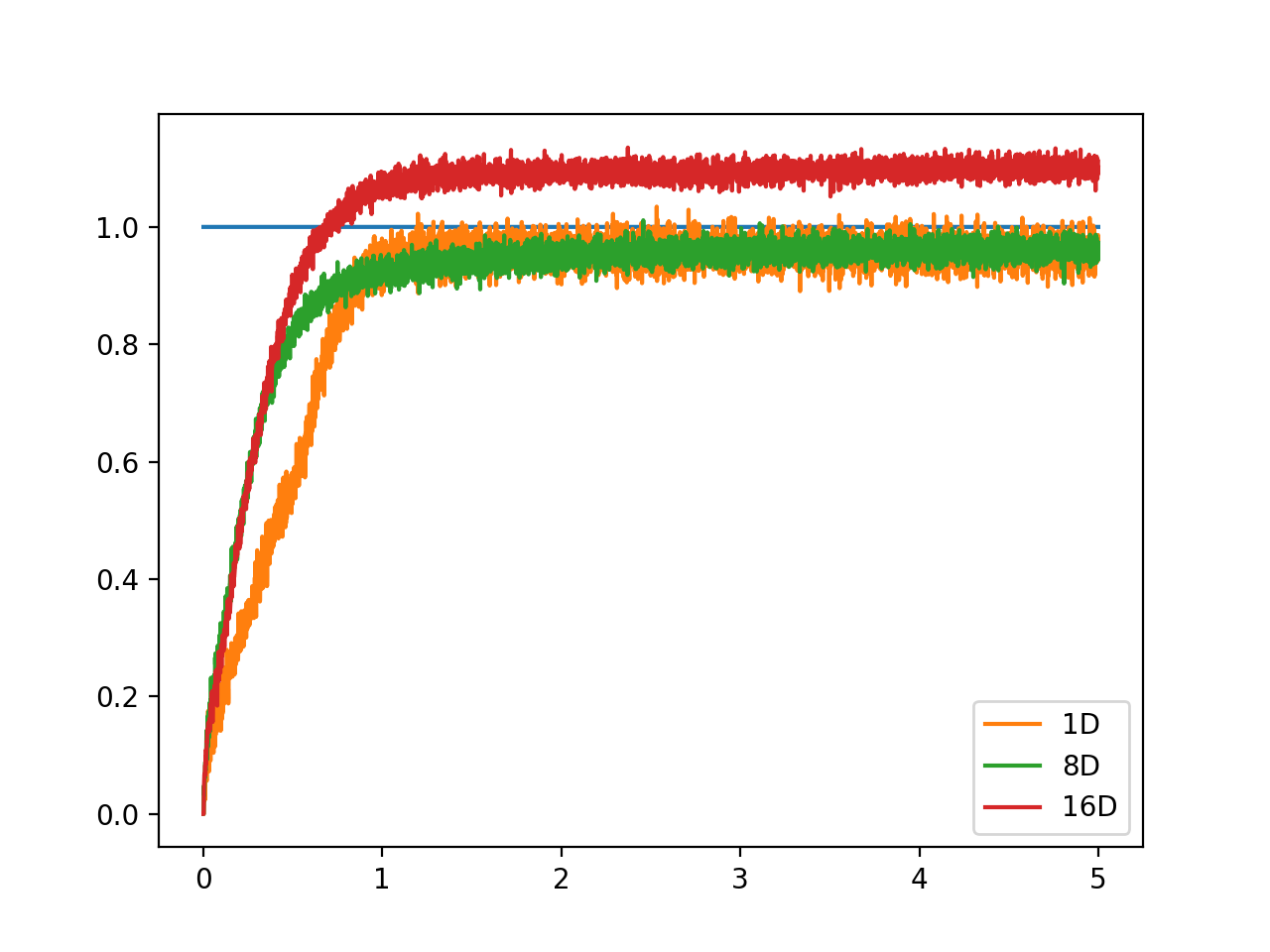
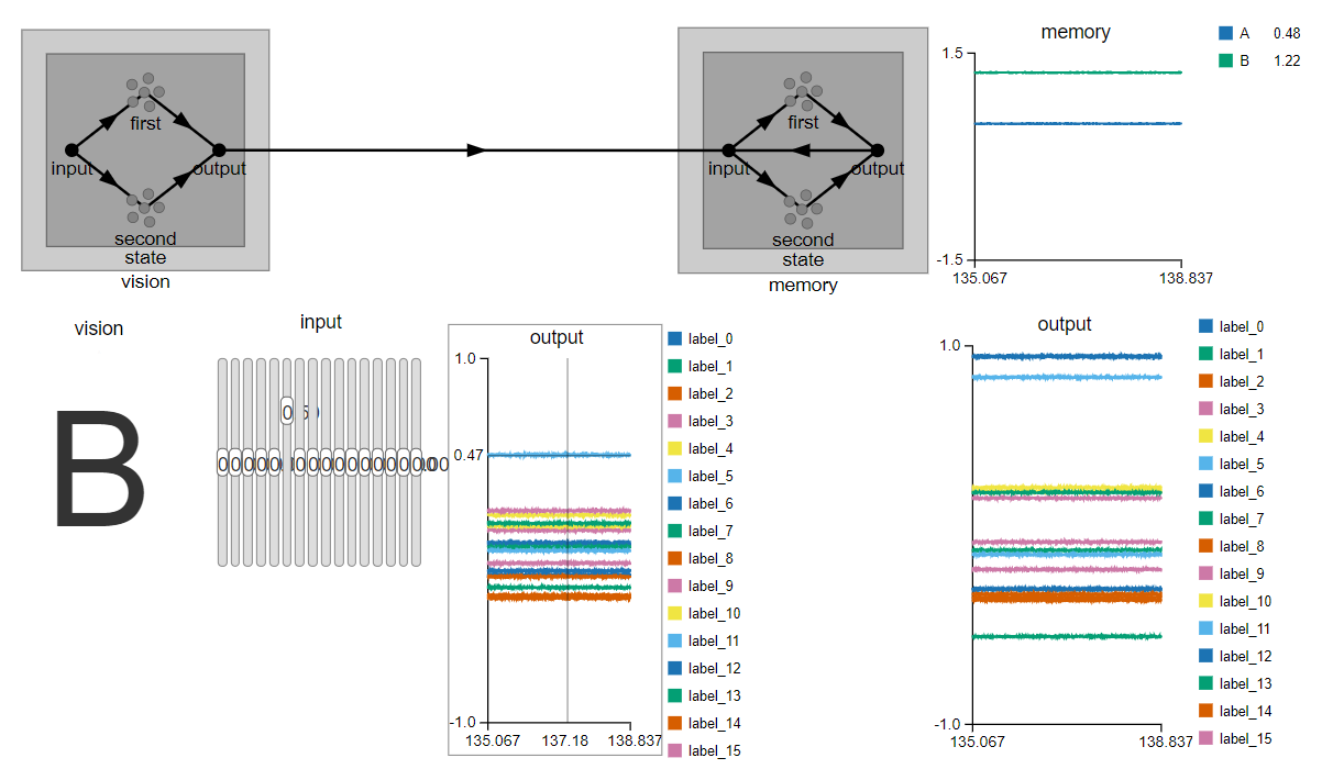
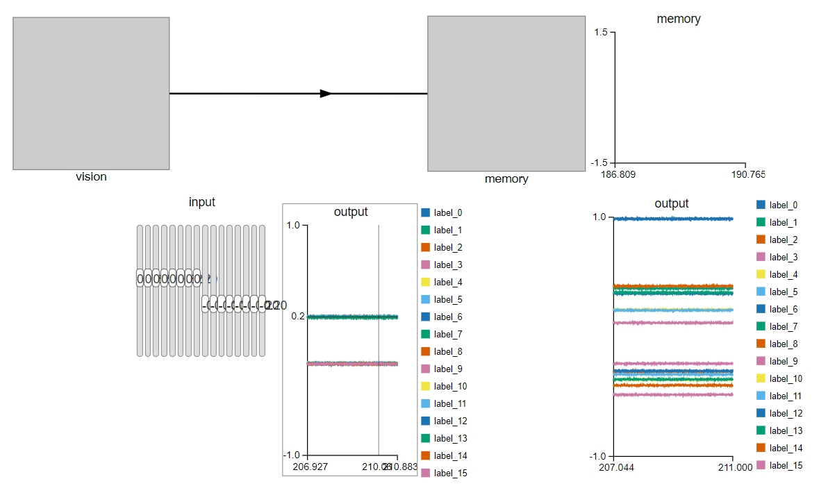
As a side note, I’m not 100% sure why, but as you increase the number of dimensions, the maximum “saturated” value represented by the integrator can actually increase as well. Below is a comparison of the vector norm of an output vector stored in several multi-dimensional integrators (1D, 8D, 16D). Each integrator is feed with a constant input of a vector projected along the x-axis.

Note: The plot below is a rather extreme example. The “saturation” value of the 8D and 16D generally ranges from about 1.1-1.3.

image

Here is the code:

import numpy as np
import nengo
import matplotlib.pyplot as plt

tau = 0.1

with nengo.Network() as model:
    in_node = nengo.Node(lambda t: 1)

    ens1 = nengo.Ensemble(50, 1)
    ens2 = nengo.Ensemble(50 * 8, 8)
    ens3 = nengo.Ensemble(50 * 16, 16)

    nengo.Connection(in_node, ens1, transform=tau)
    nengo.Connection(ens1, ens1, synapse=tau)
    nengo.Connection(in_node, ens2[0], transform=tau)
    nengo.Connection(ens2, ens2, synapse=tau)
    nengo.Connection(in_node, ens3[0], transform=tau)
    nengo.Connection(ens3, ens3, synapse=tau)

    pi = nengo.Probe(in_node)
    p1 = nengo.Probe(ens1, synapse=0.01)
    p2 = nengo.Probe(ens2, synapse=0.01)
    p3 = nengo.Probe(ens3, synapse=0.01)


with nengo.Simulator(model) as sim:
    sim.run(5)


norm1 = np.linalg.norm(sim.data[p1], axis=1)
norm2 = np.linalg.norm(sim.data[p2], axis=1)
norm3 = np.linalg.norm(sim.data[p3], axis=1)

plt.figure()
plt.plot(sim.trange(), sim.data[pi])
plt.plot(sim.trange(), norm1, label="1D")
plt.plot(sim.trange(), norm2, label="8D")
plt.plot(sim.trange(), norm3, label="16D")
plt.legend()
plt.show()

I hope that helped! :smiley:

Short comment/question regarding the maximum represented value in an N-D integrator. Can it be that it increases because the radius of the ND sphere inscribed in the ND-cube slightly increases with number of dimensions? https://en.wikipedia.org/wiki/Volume_of_an_n-ball

Hmm. That may be a possibility, although I’d have to do some more investigation before I can present a definitive answer. It may also be a quirk of how we choose (i.e., the distribution of) the evaluation points in higher dimensions, or the way the decoders are solved, or even how the encoders are distributed (which affects the number of neurons that respond to a given input vector)… This requires some thought. :thinking:

I don’t think the radius of the ND sphere increases, it should stay constant and equal to half the side length of the ND cube. However, the relative volume close to the surface increases while the relative volume close to the center shrinks. This probably explains part of the effect because Nengo distributes the intercepts uniformly by default and thus we get much more neurons firing for values close to the edge of the representational space (and that are not as saturated for values in that area). This can be counteracted by using intercepts=nengo.dists.CosineSimilarity(d + 2) (d is the dimensionality), which nengo_spa.State uses. Adding this to the example above, the plot looks like this:

A second effect is that the evaluation points used for the optimization of the decoders fail to cover the outer bounds of the ND sphere because this area/volume is not in the convex hull of the evaluation points.
Screen Shot 2020-09-27 at 17.32.59

You migth want to take a look at chapter 6 of my thesis which touches on some of these aspects.

1 Like

Wow, thank you for this little research @xchoo! :grinning:
Sorry for such a long time without an answer…

I’ve analyzed your first example (integrator vs ramp) and your explanation. It’s surprising for me, to think about a neural integrator as a bunch of fixed points and pushing the “state” between them. I think it’s a great intuition, thank you for that!

But… I was still confused - my observation was: if I feed one dimension of the State object with some value (0.2 for example), it will reach this value (0.2) and stay there (it looks similar in the GUI when setting state with Semantic Pointer Cloud - after a closer look, it actually looks different, but still not clear). Instead, if I feed this “low-level”, self-made integrator with the same value, it will saturate to about 1. So I decided to check it by modifying your code and feeding integrators with 0.2. I was surprised - State object (with many neurons per dimension, to avoid sticking to fixation points) behaved exactly the same as the self-made integrator - it saturated around 1. My hypothesis was wrong. You can see the code and the figure below:

import time
import nengo
import nengo_spa as spa
import matplotlib.pyplot as plt

sim_time = 10

with spa.Network() as model:
    neuron_type = nengo.LIFRate()
    nn = 500
    radius = 1

    seed = int(time.time())
    print("Using seed: ", seed)

    ramp_scale = 0.2
    ramp = nengo.Node(lambda t: t * ramp_scale)
    level = nengo.Node(ramp_scale)

    ens_ens = nengo.Ensemble(nn, 1, seed=seed, neuron_type=neuron_type, radius=radius)
    nengo.Connection(ramp, ens_ens)

    tau = 0.1  # Feedback synapse for the integrator
    int_ens = nengo.Ensemble(nn, 1, seed=seed, neuron_type=neuron_type, radius=radius)
    nengo.Connection(level, int_ens, transform=tau, synapse=tau)
    nengo.Connection(int_ens, int_ens, synapse=tau)

    state = spa.State(16, feedback=1, feedback_synapse=tau, neurons_per_dimension=nn)
    nengo.Connection(level, state.input[0], transform=tau, synapse=tau)

    p_ramp = nengo.Probe(ramp)
    p_ens = nengo.Probe(ens_ens, synapse=0.01)
    p_int = nengo.Probe(int_ens, synapse=0.01)
    p_state = nengo.Probe(state.output[0], synapse=0.01)

with nengo.Simulator(model) as sim:
    sim.run(sim_time)


plt.figure()
plt.plot(sim.trange(), sim.data[p_ens], label="ens")
plt.plot(sim.trange(), sim.data[p_int], label="integrator")
plt.plot(sim.trange(), sim.data[p_ramp], 'k--', label="ramp")
plt.plot(sim.trange(), sim.data[p_state], label="state")
plt.plot([0, sim_time], [radius, radius], 'r--')
plt.ylim(0, 2)
plt.legend()
plt.show()

Figure_1

So what’s wrong? Please look at the screenshots below. When using GUI with state objects (with many neurons per dimension) and Semantic Pointer Cloud, something strange happens - some values of a vector which comes out of the first state object are much bigger than 0.2, but mostly they won’t saturate in memory (label 5 at about 0.35 is not saturated in memory, red labels at about -0.30 also).

import nengo
import nengo_spa as spa

nn = 500
dimensions = 16
tau = 0.1
model = spa.Network()
with model:
    vision = spa.State(dimensions, neurons_per_dimension=nn)
    memory = spa.State(dimensions, neurons_per_dimension=nn,
                       feedback=1, feedback_synapse=tau)
    nengo.Connection(vision.output, memory.input, transform=tau)

I can additionally modify them with input sliders and they still won’t saturate (label 5 at 0.47 is equal about 0.8 in memory).

So, I tried to use state objects without Semantic Pointer Cloud, using only sliders set to 0.2 or -0.2, and here the next surprise comes - each time I do the test, only the first dimension behaves as a standard integrator (saturates) - others don’t:

So, I’ve checked again the first example attached to this post, but this time I’ve used other dimensions. Sometimes it saturates (but not so clearly like the first dimension), sometimes sticks to point below 1.

My conclusion: the first dimension of a state object behaves like a standard, one-dimensional integrator. Other dimensions behave differently. It’s a bit mindblowing for me :joy:. Is there any explanation for such behaviour in the implementation? :grinning:

The first dimension of a State does indeed behave differently. In general, the State internally splits up the representation into multiple ensembles of lesser dimensionality to improve build performance and accuracy. The intercepts of these ensembles are chosen to support the representation of high-dimensional unit vectors and thus will tend to saturate at a radius below 1. However, the first dimension is handled separately gets an ensemble all by itself that uses normal intercepts and radius, so that the first dimension will saturate around 1 (it’s integration behaviour will also be more stable).

You’ll probably wonder, why the first dimension is handled is this special way. When manipulating Semantic Pointers with Holographic Reduce Representations (HRRs)/circular convolution, there are certain instance where you will have to represent the identity vector (i.e. the vector that does not change a Semantic Pointer when bound to it); @xchoo might have a concrete example of such a situation. The identity vector for circular convolution is (1, 0, 0, 0, ....) and to accurately represent it, we need to treat the first dimension in State accordingly.

This special treatment might not always be desirable (e.g. when doing learning between states because it complicates the network structure) and thus can easily be switched off with State(represent_cc_identity=False). (I think you can also set that globally with the Nengo config system, but would have to look up the exact syntax.l)

Some references:

1 Like

Oh, so it’s a bit more tangled… Ok, that answers my question. Mathematically a bit complicated for me, but I’ll dive into (thanks to the references).

Thank you very much! :grinning:

Yup! As @jgosmann said, the first dimension of the spa.State network is treated differently than the other dimensions in the vector. To understand why this is the case, we need to understand how the spa.State network itself is structured.

** For the purposes of the discussion below, I’m going to set represent_cc_identity to False until it’s used.

What Nengo does when it builds a spa.State network

Using the default parameters, a spa.State network is created with several sub-dimensions. So, if you create a 64-dimensional State for example, instead of creating a 64D ensemble, it creates four 16D ensembles:

with spa.Network() as model:
    state64 = spa.State(64, represent_cc_identity=False)

looks like this:

The effect of subdimensions on build time

The primary reason why this is done is for speed. If the spa.State were to use one giant N-dimensional ensemble, it would have $N \times num–neurons–per–dim$. The time it takes to build an ensemble of neurons increases exponentially. Here’s an example of how the build time increases with the number of neurons in an ensemble:
test_ens_build_time.py (394 Bytes)

4D NN=200 Build time: 0.1025s
8D NN=400 Build time: 0.2028s
16D NN=800 Build time: 0.3036s
32D NN=1600 Build time: 0.8142s
64D NN=3200 Build time: 3.0503s
128D NN=6400 Build time: 15.2367s
256D NN=12800 Build time: 149.3669s

The effect of subdimensions on integrator stability

However, using multi-dimensional ensembles to build a spa.State network does have a disadvantage. When used as an integrator, a State with multi-subdimensional ensembles is less stable than a State with single-subdimensional ensembles. As an example, the following code compares a 64D spa.State using 1, 2, 16, and 64 dimensions as the number of subdimensions:
test_spa_mem_stability.py (1.9 KB)
image

The effect of subdimensions on vector inputs greater than 1

Okay! So now we know that to increase stability of spa.State integrators, we should reduce the number of subdimensions in the spa.State network. But that begs the question, why not use subdimensions=1 for every spa.State? Well, this is because we can use multi-dimensional ensembles to sort of “normalize” vectors. In this code, a 64D spa.State with 1, 2, 16, and 64 subdimensions each have an input vector that increases in vector magnitude over time.
test_spa_saturation.py (1.9 KB)
image

As you can see in the plot, as you increase the size of subdimensions, the “normalization” effect of the ensemble gets better. Considering all of the various factors (build speed, memory stability, vector “normalization”), we settled on 16 subdimensions as a default.

The represent_cc_identity parameter

So… that was a pretty long explanation, but we’ve only discussed why we use 16 as the default subdimension value. What about the represent_cc_identity parameter? What is that used for?
In order to understand that, we must understand how SPA vectors are created, as well as a special SPA vector known as the Identity vector.

SPA vectors created (by default) have a special property. The individual vector elements have an expected value of $-\frac{1}{\sqrt{D}}$ to $\frac{1}{\sqrt{D}}$, where $D$ is the dimensionality of the vector. That’s all fine and dandy in typical situations since NengoSPA takes this into account. However, there is one special vector that where this assumption doesn’t hold, and that is of the identity vector (i.e., a vector like this [1, 0, 0, ...., 0]). For this specific vector, all elements except the first are 0, and the first element is 1 (which is definitely much much bigger than $\frac{1}{\sqrt{D}}$, especially if $D$ is a large number like 512).

So… what implications does this have for NengoSPA? Well, if you are trying to represent the identity vector using a spa.State network, then the specifics of the network affect how well you can represent this vector. As an example, this is a 1, 16, 64 and 512D spa.States with subdimensions=1 trying to representing the identity vector. The output plot shows the value of the first vector element being represented.
test_spa_identity.py (940 Bytes)
image

And as you can see from the plot, as the dimensionality of the spa.State network grows, it’s ability to represent the special identity vector diminishes. We can perform this experiment using subdimentions=16:
image

and subdimensions=64:
image

and we see that as long as subdimensions < dimensions, we have this issue. So… how to we get around this issue and support the representation of the identity vector? Well, that’s where the represent_cc_identity parameter comes in. It treats the first element of the vector as a special case and creates its own special ensemble, independent of the rest of the other vector elements.

Why is the identity vector important?

So… we go through all of this trouble just so that we can represent the identity vector. But, why is it important? Can we just not use the identity vector, and make our lives simpler? As it turns out, the identity vector is especially useful, particularly when performing SPA-algebraic operations that result in duplications of the input.

Let’s do an example in standard algebra. Suppose I had a variable “A”, and I wanted to multiply it with something to get the result “A + AB” (i.e., a copy of itself, plus a mutated version of itself). What would this operand be? It would be (1 + B).

The identity vector allows us to perform this sort of operation but in vector space. If I had a semantic pointer A, and I wanted to compute a result that is A + AB, I would need to do the following vector binding operation: $A \circledast (I + B)$, where $I$ is the identity vector.

If you want to know more about this, you can read my thesis, specifically, section 4.3.2. :smiley:

1 Like

Wow, thank you very much! It’s very intuitive explanation - you’re a great teacher :grin:

Thanks again, it’s much clearer now, especially thanks to the sections about vector normalization and identity vector :smiley: :+1: