Nengo NEF algorithm. Finding gain and bias

I am learning Nengo and NEF and going through the examples in the tutorials.

In the example, it shows the algorithms to find the gain and bias for LIF neurons but I don’t get the logic behind it. (z, g, b etc).

Could someone explain the formula a little bit more?

Thanks,

Hi @corricvale, and welcome to the Nengo forums! :smiley:

The piece of code you are asking about converts a pair of intercept and rate values into the gain and bias values needed for the LIF neuron (other neurons have similar functions, but the code you posted is specifically for the LIF neuron).

To understand what is going on, we have to step back a bit. First, understand that a crucial part of the neural network is how a neuron functions. The neurons in the Nengo networks essentially (and this is at a high level) map a specific input current to a firing rate. I.e., if you feed that neuron a specific amount of input current, the neuron will spike at a specific rate. To calculate the input current ($J$) to a neuron, we use the formula:

$J(x) = \alpha x + J_{bias}$

where $\alpha$ is some gain value, and $J_{bias}$ is some bias current (a constant unchanging current being fed into the neuron).

With this input current, the firing rate ($a$) of an LIF neuron is computed as such:

$a(x) = \frac{1}{\tau^{ref} - \tau^{RC}ln(1 - \frac{J_{th}}{J(x)})}$

where $\tau^{ref}$ and $\tau^{RC}$ are the refractory and membrane time constants of the LIF neuron, respectively; and $J_{th}$ is the firing threshold current for the neuron (typically set to 1 for simplicity).

If you plot the firing rate of the LIF neuron over a range of inputs $x$ (i.e., you take $x$, compute $J$, then compute $a$), you get a graph that has a shape like the following:

image

Note that the various values for $\tau$s, and $\alpha$ and $J_{bias}$ all affect the shape of this curve.

Now, back to your question, what does the code you posted do?
In Nengo, there are two ways to specify the shape of the neuron firing curve (also called the neuron’s response curve). The first is by specifying the gain and bias values manually, and you can do so in Nengo’s ensemble class creation (see docs here). However, this method is not very intuitive if you do not have a good understanding of how the gain and bias values will affect the shape of the neuron response curves.

The other method is to specify two known points on the desired neuron response curve and work backwards to figure out the gain and bias values. For an analogous problem, it’s like finding the slope and intercept of a line given two points that the line must pass through. This is what the code you posted is doing. It re-arranges the activity and input current formulae to find the gain and bias values that will meet the specified intercept and firing rate values.

Nengo & NEF Learning Materials
If you are looking for additional Nengo and NEF learning materials, I recommend you check out this YouTube playlist! The formulae and concepts I discuss above is (if I recall correctly) discuss in Lecture 2. :smiley:

1 Like

Thanks for the explanation xchoo.

I went through the youtube lectures and I understand the concepts but still am not sure how the equations are derived.

I can see that z is the input current (J) when the neuron is at the desired maximum rate and hence b = 1 - gintercept according to J = alphax + Jbias.
However, I dont get how g = (1 - z) / (intercept - 1.0) has been derived.

Could you explain a little bit more?

Thanks!

Righto. I can see your confusion, the equation derivation is a little more nuanced than just the equations for $J$ and $a(x)$. Btw, our forums support $\LaTeX$. Simply encapsulate a $\LaTeX$ formula within $, like so:

$\LaTeX$

Back to the explanation!
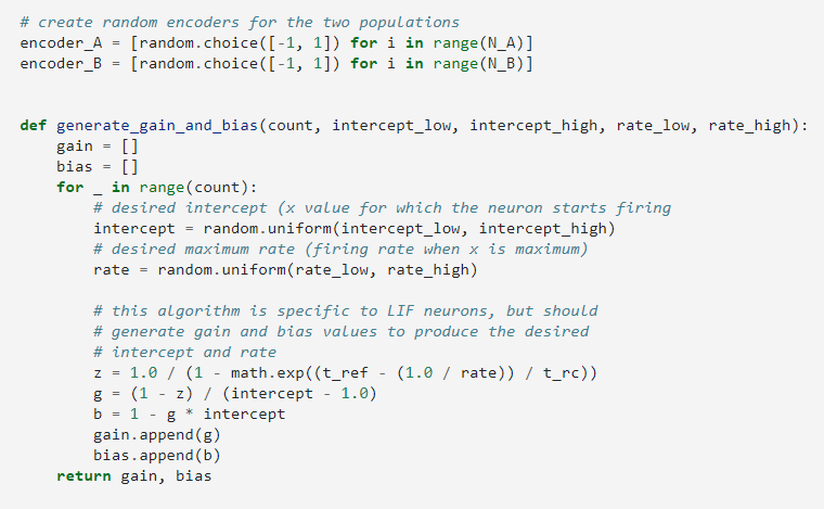
So, as I mentioned before, there are two equations that map the neuron gain ($\alpha$) and neuron bias current ($J_{bias}$) to the firing rate ($a$) of an LIF neuron. We have:

$J(x) = \alpha x + J_{bias}$ (Eq. 1)

which converts an input value $x$ to the neuron input current $J(x)$. And we also have the LIF activation function:

$a(x) = \frac{1}{\tau^{ref} - \tau^{RC}ln\left(1 - \frac{J_{th}}{J(x)}\right)}$

We can re-arrange the activation function to solve for $J(x)$ like so:

$J(x) = \frac{J_{th}}{1 - e^{\left(\frac{\tau^{ref} - \frac{1}{a(x)}}{\tau^{RC}}\right)}}$

If you look at the code, this is what z is computing. Before continuing, I would like to clarify out that the following statement is slightly incorrect:

Rather, z computes the input current for the neuron given any value of the rate $a(x)$ (doesn’t have to be the maximum rate).

With the two equations for $J(x)$, we notice that without additional information, they are insufficient to actually solve for $\alpha$ and $J_{bias}$. So… how do we actually do this? As with solving for $m$ (slope) and $c$ (constant) for an equation of a straight line, we need two known fixed points!

The First Point
The first known point is for the intercept value. When $x = intercept$, by definition, the firing rate of the neuron is 0. This doesn’t help much because substituting $a(x_{intcpt}) = 0$ into $J(x)$ causes the equation to blow up (we have a division by 0 in the equation). But, by definition, when the neuron is at that firing threshold, we know that the input current to the neuron $J(x)$ must be equal to the threshold firing current $J_{th}$ of that neuron. Using this fact, and Eq. 1, we can then write:

$J_{th} = \alpha x_{intcpt} + J_{bias}$

In Nengo, we set $J_{th} = 1$ (it’s arbitrary, and a simple value to work with), so,

$1 = \alpha x_{intcpt} + J_{bias}$ (Eq. 2)

The Second Point
The second fixed point is the “maximum” firing rate of the neuron. I must clarify that there are two “maximum” rates for the neurons in the NEF. The “true” maximum is basically how fast the neuron will fire given an infinite input current. This is basically $1 / \tau^{ref}$ (i.e., producing a spike the instant the refactory time is up). This value is not helpful to us in this derivation, so that’s all I’ll say about it for now.

The other “maximum” value is a definition of how fast we want the neuron to fire at some maximal $x$ value. In the NEF, the input values for $x$ are assumed to be within -1 to 1, and hence, the “maximum” firing rate of the neuron is defined to be when the input $x = 1$. With this, we can re-write Eq. 1 as:

$J(1) = \alpha + J_{bias}$ (Eq. 3)

Solving for $\alpha$ and $J_{bias}$

With Eq. 2 and Eq. 3, we can now solve for $\alpha$ and $J_{bias}$ by doing a bit of algebra. First, we rearrange Eq. 3 to solve for $J_{bias}$:

$J_{bias} = J(1) - \alpha$ (Eq. 4)

And we substitute into Eq. 2 to solve for $\alpha$:

$1 = \alpha x_{intcpt} + J(1) - \alpha$
$1 - J(1) = \alpha(x_{intctp} - 1)$
$\alpha = \frac{1 - J(1)}{x_{intctp} - 1}$

If you look at the code, this is what g is computing.
And once we have $\alpha$, we can solve for $J_{bias}$ by substituting into Eq. 2:

$1 = \alpha x_{intcpt} + J_{bias}$
$J_{bias} = 1 - \alpha x_{intcpt}$

And if you look at the code, this is what b computes. :smiley:

Afternotes
I should note that this method for solving for $\alpha$ and $J_{bias}$ is applicable to other neuron types (i.e., not LIF neurons) as well. All you would have to do is replace the current equation $J(x)$ with the current equation for the other neuron type.

1 Like

Hello @corricvale, adding to the above excellent explanation by @xchoo, I think you might this resource useful to understand the dynamics of the LIF neuron. As you would see in the simulation phase, an input of $J_{th}=1$ the LIF neuron’s voltage although seemingly reaches to the threshold of 1, it fails to spike!, thus 0 firing rate as is being explained here.

Thank you xchoo for your great explanation.

May I ask one more question if you don’t mind?

The tunning curve generated by the above method gives somewhat “noisy” tunning curve as shown below
examples_advanced_nef-algorithm_9_0

However, when I was using Nengo GUI’s “Draw tunning plot feature”, the graph was much more smooth.

Is this because the example in the tutorials is more simpler methods, presented for the teaching purpose, than what Nengo actually does in the backends?
Or is it because the tunning curve plot in Nengo Gui is the filtered plot of the raw tunning curve?

Thanks for your great help!

Thanks zerone.

I will go through it.

Hi @corricvale, with regards to your question:

Yes! There is a difference between how the tutorial code is generating the tuning curves for the ensembles versus how Nengo does it. In the tutorial code, two factors compound to generate the “noisy” nature of the tuning curves.

First, in the tutorial, the firing rate of a neuron is calculated by running the neuron for a short amount of time (0.5s), and then counting the number of spikes generated in that time frame. Because the spikes are only collected within this small time window, a difference of 1 or 2 spikes makes a large difference in the computed spike rate. E.g., 10 spikes in 0.5s is 20Hz, whereas 11 spikes in 0.5s is 22Hz, and this difference is large enough to show up as a bump on the plot.

Second (and this is a compounding issue) is that for the simplistic neuron model implemented in the tutorial, neurons can only generate spikes within 1 dt (timestep) of the simulation. After a spike is generated, the neuron is reset for some refractory period that is aligned with the timesteps of the simulation. As an example, suppose that for a given input current, a neuron is to fire every 33ms (0.0033s). With the simulation dt of 0.001s, the neuron can only fire at t=0.004s, t=0.008s, … vs t=0.0033s, t=0.0066s, t=0.0099s. This means that with the simplistic neuron model, spike times that don’t fall neatly on the boundaries of dt have the effect of “smudging” the actual firing rate. This combined with the previous factor leads to the spikiness you observe in the plot.

The tuning curves generated by the NengoGUI plot is smooth because it uses the rate-based approximation of the LIF neuron to plot the curve (i.e., the curve is generated using the equation for $a(x)$, rather than by recording spikes from a running simulation).

As a side note, the LIF neuron model implemented in Nengo also contains some logic to better calculate the actual spike time, rather than relying on the dt boundaries to determine when the neuron should reset / fire next.

1 Like