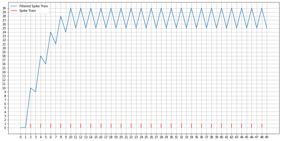
Upon applying a Lowpass synaptic filter to a spike train as in the following code, one can see that the smoothed output rises initially and then it stabilizes. Why is that so? If you have spikes at regular intervals (e.g. every 7th time-step), shouldn’t the smoothed output keep rising as long as the spikes are passed to the filter? Does the smoothed output stabilize around a value because of the extremely low values at the tail of the filter? Please let me know.
Um… No, it’s quite the opposite actually.
The output stabilizes because the the exponential filter that is applied decays so quickly that the tail goes to 0 pretty fast.
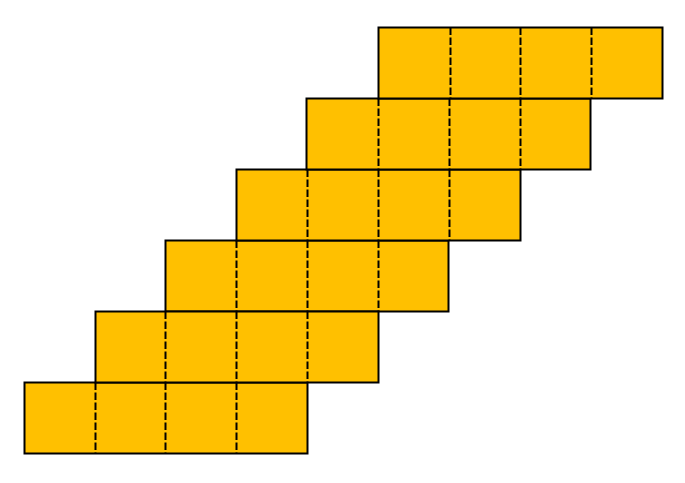
Lets consider a simpler example: instead of the exponential signal, let’s instead use a 4dt rectangular pulse. The pulse goes to some arbitrary value, and stays there for 4 timsteps, after which it goes to 0 (i.e., it goes to 0 quite quickly). Now lets see what happens for a train of spikes, with 1 spike every timestep. For each spike, we add this rectangular pulse to the output signal (the output signal starts at 0). You think you’d expect something like this:
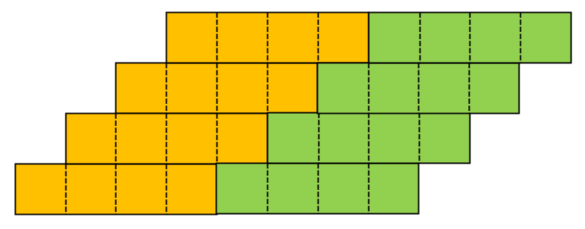
Where the output signal goes 1, then 2, then 3, then 4, then 5, and increases monotonically, but… if you look closer, you’ll see that there is a lot of space under the curve starting at the 5th timestep. In fact, the output of the signal (in this simplified example) is the sum of the number of squares in each column, which would be 1, then 2, then 3, then 4, then 4 (and 4 ad infinitum)! This shows that the output ramps up, then stabilizes, even if we apply the 4dt pulse filter to each spike. You can visualize the actual output shape by redrawing the figure about like so, where the different colours denote different “groups” of repeating filters:
And as before, we see that the output ramps up to 4 then stabilizes.
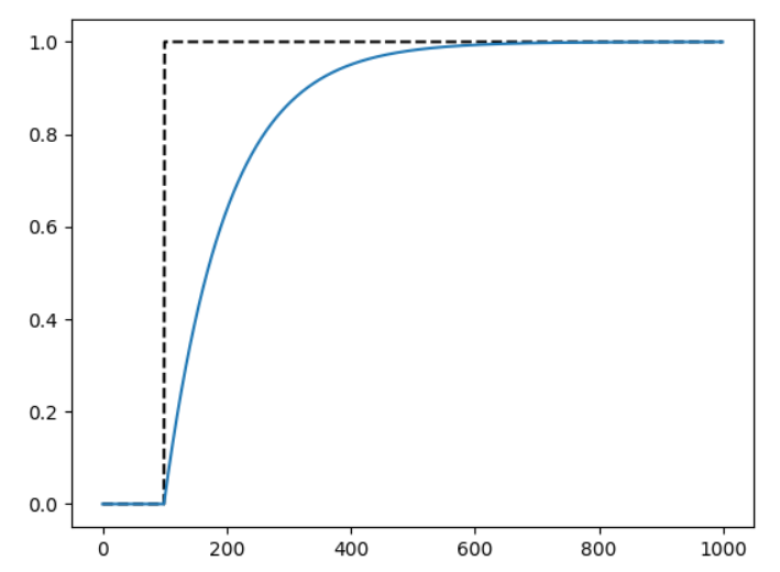
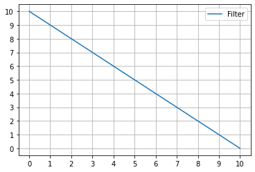
The one thing the synaptic filter does affect though, is the shape of the ramp. For the exponential synapse, it effectively low-pass filters the signal, smoothing out any shape corners, and it turns a step function (the dashed line in the plot below) into something like this:
Incidentally, this is the same shape you see in your plot above. In your plot, the output is “spikey” because the spikes are far enough apart to show the gaps between each spike. If you were to have it so that the neurons were spiking infinitely fast, all of the spikes combined forms a step function, and when lowpass filtered, the step function turns into the output above!
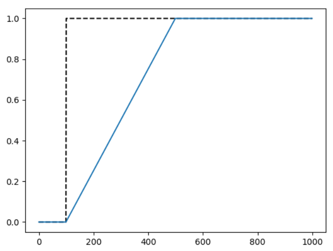
Similarly, the pulse filter (in the simple example above), turns a step function into a ramp with a maximum value like this:
And, if we were to take the example above, and shrink the dt to an infinitesimally small size (i.e., you make each “square” smaller and smaller), you can sort of see the stacked squares turning into the “ramp + flat top” graph you see above!
To Summarize:
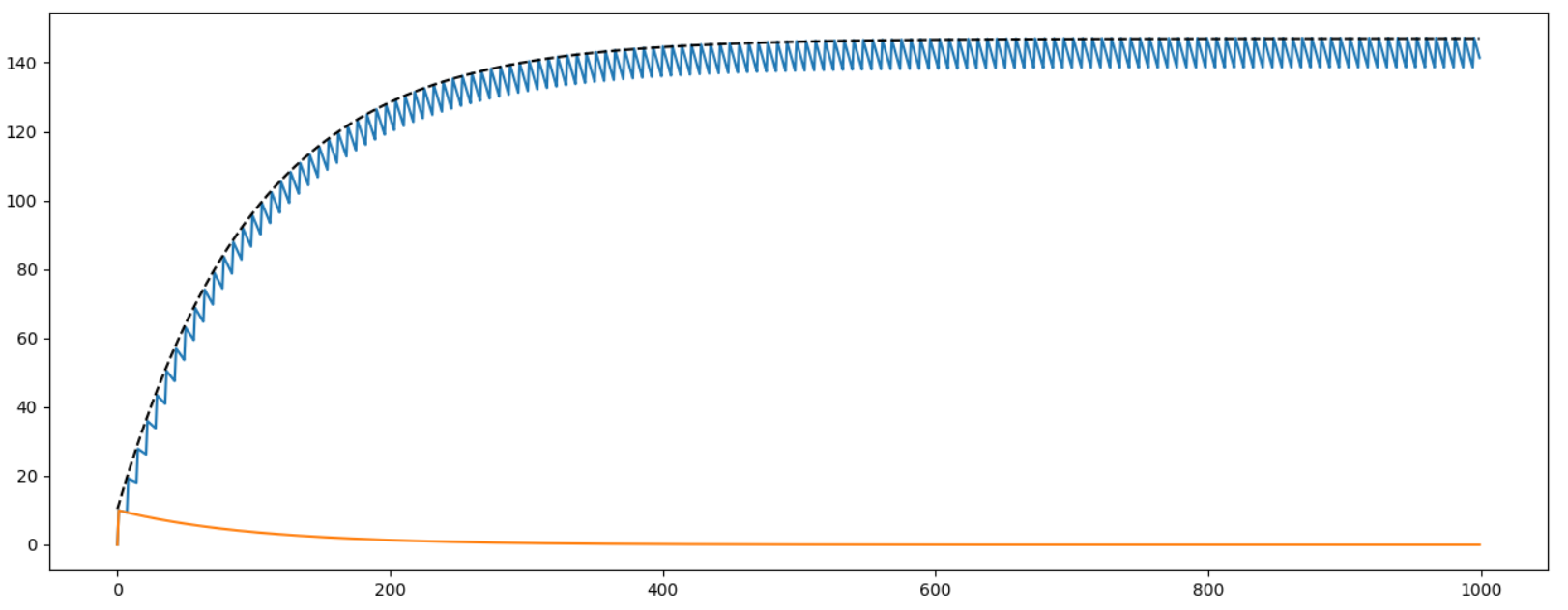
The output of the filtered spike train “levels off” precisely because the exponential filter that is applied decays to 0 after some time. When it decays to 0, it no longer contributes to the output signal. Since it decays to 0 in a finite amount of time, even if you add up an infinite sequence of these filters, you will have the output stabilize to some value (eventually). You can get a sense of this by plotting the output of the filtered spike train against 1 single instance of the exponential filter:
You can see from the graph above that as the first exponential filter decay, it’s contribution to the output decreases, and so does the “peak” value (the black dashed line) of the output signal.
The rate at which the filter decays to 0 determines how long the output will need to stabilize. Increasing the filter time constant (which makes the tail longer) increases the amount of time it takes for the signal to reach steady state, and vice versa for shorter time constants. This plot is, for example, with a time constant of 0.1s (changing no other parameters in the code):
I got this @xchoo, not sure how I missed it. A simple calculation on pen and paper would have been sufficient. The increment in filtered signal after every timestep when the spike occurs decreases in case of exponential filter (or a filter with downward slope as shown below) or remains constant in case of rectangular pulse. Although soon the subsequent increment in the filtered output goes to 0 for a decaying filter or becomes exactly 0 for a rectangular pulse, and then the filtered signal fluctuates due to previously accumulated values at the tail end of the filtered signal. Thanks!
spike_train_idcs = []
for i in range(spike_train_len):
    if A[i]==1: # i.e. a spike is here.
        spike_train_idcs.append(i)

plt.figure(figsize=(16, 8))
plt.plot(A_filtered, label="Filtered Spike Train")
plt.vlines(spike_train_idcs, 0, 1, color="red", label="Spike Train")
plt.yticks(range(31))
plt.xticks(range(spike_train_len))
plt.legend()
plt.grid()
One of the properties of the convolution operation is that when you convolve a filter with an unit impulse (or a spike), what you get out is a replica of the filter. If you have a train of impulse functions, you get one replica of the filter at the location of each spike (added together, of course).