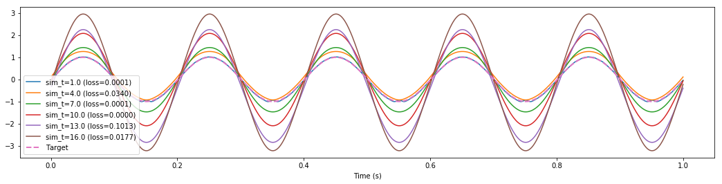
I’m encountering this behaviour that I’m finding difficult to debug / understand, where longer training simulations (i.e., more training data) of the exact same network effectively rescales the output and degrades performance significantly.
The weird thing about this is the loss reported by nengo_dl is not changing by any significant amount. In fact it seems uncorrelated with the MSE that I calculate offline from the exact same data (see print statements at end of post). The offline MSE mirrors what you would expect by visually inspecting the attached plot, while the loss reported by nengo_dl seems arbitrary.
Maybe I’m misunderstanding some nuances surrounding the optimization hyperparameters / how the MSE is reported / how the parameters are carried over? How can I get consistent performance across different lengths of training time?
Details: I’m trying to learn a function from $\mathbb{R} \mapsto \mathbb{R}$ by using backprop to optimize both the encoders and decoders, with a single layer of sigmoidal units in between (i.e., a standard perceptron). The example function is just the identity (i.e., communication channel). Training and testing uses the same 5 Hz sinusoid in all conditions. RectifiedLinear units produce approximately the same behaviour.
import numpy as np
import matplotlib.pyplot as plt
import seaborn as sns

import nengo
from nengo.utils.numpy import rmse

import nengo_dl
import tensorflow as tf


def go(sim_t,
       n_neurons=100,
       freq=5,
       n_epochs=100):

    with nengo.Network(seed=0) as inner:
        tf_input = nengo.Node(output=np.zeros(1))

        u = nengo.Node(size_in=1)
        x = nengo.Ensemble(n_neurons, 1, neuron_type=nengo.Sigmoid())
        y = nengo.Node(size_in=1)

        nengo.Connection(tf_input, u, synapse=None)
        nengo.Connection(u, x, synapse=None)
        nengo.Connection(x, y, synapse=None)

        tf_output = nengo.Probe(y, synapse=None)

    t = np.arange(0, sim_t, 0.001)
    data_y = np.sin(2*np.pi*freq*t)[:, None]
    data_u = data_y
    inputs = {tf_input: data_u[:, None, :]}
    outputs = {tf_output: data_y[:, None, :]}

    with nengo_dl.Simulator(inner, minibatch_size=100) as sim_train:
        optimizer = tf.train.AdamOptimizer()
        sim_train.train(inputs, outputs, optimizer, n_epochs=n_epochs, objective='mse')
        sim_train.freeze_params(inner)
        loss = sim_train.loss(inputs, outputs, 'mse')

    with nengo.Network() as outer:
        test_input = nengo.Node(output=nengo.processes.PresentInput(data_u, sim_train.dt))
        outer.add(inner)
        nengo.Connection(test_input, u, synapse=None)
        test_output = nengo.Probe(y, synapse=None)

    with nengo_dl.Simulator(outer) as sim:
        sim.run(sim_t)

    return {
        't': sim.trange(),
        'actual': sim.data[test_output],
        'target': data_y,
        'loss': loss,
    }

try_sim_t = np.linspace(1, 16, 6)
data = []
for sim_t in try_sim_t:
    data.append(go(sim_t=sim_t))

sl = slice(1000)
plt.figure(figsize=(18, 4))
for sim_t, r in zip(try_sim_t, data):
    plt.plot(r['t'][sl], r['actual'][sl],
             label="sim_t=%s (loss=%.4f)" % (sim_t, r['loss']))
    print("sim_t=%s (mse=%s)" % (
        sim_t, rmse(r['target'].squeeze(), r['actual'].squeeze())**2))

# all of the targets are the same (only differs in length)
plt.plot(r['t'][sl], r['target'][sl], ls='--', lw=2, label="Target")

plt.legend()
plt.xlabel("Time (s)")
plt.show()
Build finished in 0:00:00
Optimization finished in 0:00:00
Construction finished in 0:00:00
Training finished in 0:00:04 (loss: 0.0000)
Build finished in 0:00:00
Optimization finished in 0:00:00
Construction finished in 0:00:00
Simulation finished in 0:00:00
Build finished in 0:00:00
Optimization finished in 0:00:00
Construction finished in 0:00:00
Training finished in 0:00:16 (loss: 0.0248)
Build finished in 0:00:00
Optimization finished in 0:00:00
Construction finished in 0:00:00
Simulation finished in 0:00:01
Build finished in 0:00:00
Optimization finished in 0:00:00
Construction finished in 0:00:00
Training finished in 0:00:27 (loss: 0.0000)
Build finished in 0:00:00
Optimization finished in 0:00:00
Construction finished in 0:00:00
Simulation finished in 0:00:01
Build finished in 0:00:00
Optimization finished in 0:00:00
Construction finished in 0:00:00
Training finished in 0:00:39 (loss: 0.0000)
Build finished in 0:00:00
Optimization finished in 0:00:00
Construction finished in 0:00:00
Simulation finished in 0:00:02
Build finished in 0:00:00
Optimization finished in 0:00:00
Construction finished in 0:00:00
Training finished in 0:00:50 (loss: 0.0733)
Build finished in 0:00:00
Optimization finished in 0:00:00
Construction finished in 0:00:00
Simulation finished in 0:00:03
Build finished in 0:00:00
Optimization finished in 0:00:00
Construction finished in 0:00:00
Training finished in 0:01:02 (loss: 0.0197)
Build finished in 0:00:00
Optimization finished in 0:00:00
Construction finished in 0:00:00
Simulation finished in 0:00:03
sim_t=1.0 (mse=0.00038221049835826233)
sim_t=4.0 (mse=0.03710108930405243)
sim_t=7.0 (mse=0.10872908536932545)
sim_t=10.0 (mse=0.5926093741152001)
sim_t=13.0 (mse=1.2567356972009183)
sim_t=16.0 (mse=2.116441248688516)
FYI, this example is a stripped down version of something else that I’m working on. There, I found that a magic rescaling factor of approximately 0.13 significantly improves the accuracy of the trained network (when trained from 30 seconds of data).