Metrics Extraction with PES Learning

Hey, guys…
I have doubts about how to extract mathematical metrics from biological signals using the SNN network with PES (Supervised Learning) type learning, I intend to use it to extract signal characteristics.

My problem is to extract, for example, metrics like standard deviation, mean, maximum, minimum, among other metrics from biological signals.

To simplify my problem, I considered a simple sinusoidal input network and tried to implement the standard deviation operation. But I don’t know if I was successful.

Observation:
I know there is a difference when using ‘function’ or ‘transform’ fields in nengo.Connection(). The first behaves dynamically and the second statically. For the ‘function’ at each time step, the function described in Python is called. In ‘transform’ an optimization with numpy type operations is used. That implies processing speed, right?

Can someone help me check if I did it correctly or implement a network, using PES learning, which returns the result of the standard deviation operation of some signal, for example?

Below is my attempt to code:

import nengo
import numpy as np

model = nengo.Network()
with model:
    stim = nengo.Node(lambda t: np.sin(t * 2 * np.pi))
    pre = nengo.Ensemble(n_neurons=100, dimensions=1)
    nengo.Connection(stim, pre)
    post = nengo.Ensemble(n_neurons=100, dimensions=1)

    def init_func(x):
        # adjust this to change what function is learned
        return np.std(x)

    learn_conn = nengo.Connection(pre, post, function=init_func,
                                  learning_rule_type=nengo.PES())
    error = nengo.Ensemble(n_neurons=100, dimensions=1)

    def desired_func(x):
        return x

    nengo.Connection(stim, error, function=desired_func, transform=-1)
    nengo.Connection(post, error, transform=1)
    nengo.Connection(error, learn_conn.learning_rule)
    stop_learn = nengo.Node(1)
    nengo.Connection(stop_learn, error.neurons, transform=-10 * np.ones((100, 1)))

Awaiting return.

Hi @vzanon, and welcome back to the Nengo forums. :smiley:

I’m not entirely clear where you want to perform the analysis of these signals, so I’ll describe a few options. If you are looking to analyze the signals after the simulation has completed, the best way to do this is to use probes to obtain the signals, then use regular Python code to perform the analysis. As an example:

with nengo.Network() a model:
    ens = nengo.Ensemble(...)
    ...
    probe_ens = nengo.Probe(ens)

with nengo.Simulator(model) as sim:
    sim.run(1)

probe_data = sim.data[probe_ens]
std_data = np.std(probe_data)

Note that in the approach above, you’ll be performing the analysis on data recorded for each timestep of the simulation. If you don’t want to do this, and only use data recorded at a specific interval, you can use the sample_every parameter of the nengo.Probe to do this:

probe_ens = nengo.Probe(ens, sample_every=0.1)  # sample ens output every 0.1s

If you are looking to analyze the signal as the simulation is running, this is a little more complex. For this, the easiest is probably to put it in a nengo.Node. However, you’ll need to take into account that the function you pass to the node is evaluated at every timestep of the simulation. So, if you want to calculate something like the STD, you’ll need it to maintain a history of some sort. This forum thread has an example of how one user accomplishes this.

The last way I can think of analyzing the data is using a spiking network to perform the analysis. This is an even more complex option than using a nengo.Node since you’ll need to design a spiking network to do this. You’ll need a memory circuit to store all of the information, one set of ensemble to compute the mean, then more ensembles to perform the square function, and another ensemble to perform the summation and square root. The ensembles performing the mathematical formula to compute the STD are not too difficult to implement (it’ll be a triple layer network of ensembles), but the memory circuit to store the data points would be difficult to implement since it’ll require timing circuits to operate correctly. I would recommend not going this approach.

For nengo.Connections, this is not the case. In fact, both function and transform are used to do the same thing: solve for the connection’s weights. As an example, the following two pieces of code will result in the same connection weights:

# Connection with transform
with nengo.Network() as model:
    ens = nengo.Ensemble(30, 1, seed=1)
    out = nengo.Node(size_in=1)
    conn = nengo.Connection(ens, out, transform=2)
    p_conn = nengo.Probe(conn, "weights")

with nengo.Simulator(model) as sim:
    sim.run(0.001)
    print(sim.data[p_conn])
# Connection with function
with nengo.Network() as model:
    ens = nengo.Ensemble(30, 1, seed=1)
    out = nengo.Node(size_in=1)
    conn = nengo.Connection(ens, out, function=lambda x: 2 * x)
    p_conn = nengo.Probe(conn, "weights")

with nengo.Simulator(model) as sim:
    sim.run(0.001)
    print(sim.data[p_conn])

Functions are only evaluated at each timestep for nengo.Nodes. Functions passed to nengo.Connections are used by Nengo during the weight solving step to solve for a set of weights that approximate the desired function over a specific input range. For single dimensional values, the default range is from -1 to 1. For multi-dimensional values, the default range are points within the unit hypersphere. All this is to say that after Nengo has done the weights solving, any input value that is provided to the ensemble (that is inside the range of values) will cause the output signal of the ensemble to approximate the desired function applied to the input value. One important note about this process is that once the weights have been solved for, the weights become static, and do not change over time (unless a learning rule is applied to it).

From your code, you’ve passed the np.std function as a parameter to the nengo.Connection's function parameter. This doesn’t (probably) have the effect you want it to have. Here’s what it actually does:

  1. By doing it this way, the initial weights that Nengo puts between pre and post will approximate the result of the init_func. Ostensively, this means that when the simulation first starts, the network will “compute” the STD function on the input signal, but because there’s a learning rule applied to that connection, the weights will slowly be modified to compute the identity (y=x) function instead. What this really means is that nothing in the network ends up computing the STD function.
  2. Another issue is that the STD function is meant to be computed over a series of data points. In your code, however, the output of pre and the input to post are single dimensional. This means that Nengo will try to solve for weights that compute the STD of a single dimensional vector (because x that is passed to np.std(x) is 1D).

If I understand what you are attempting to do, I think the approach you want to take is to use the nengo.Probes to collect the data, and then perform the STD analysis on it after the simulation has completed.

1 Like

Hi @xchoo , thanks for answering my questions. It clarified a lot of information that was previously obscure. I also understood that the way I was doing it was not correct, being totally consistent with the assumptions made about the scale of the problem. I hadn’t paid attention to this feature.

Sorry for not making my request clear. But you managed to describe well what I want to do when you mention the last solution (although it is the one not recommended by you). It is about creating a network capable of storing a set of data linked to a triple layer for the respective calculation of the mean, square function, sum and root (having as output the final calculation of the standard deviation).

My idea is precisely to create subnets using Nengo capable of calculating these simple operations (addition, subtraction, multiplication, division, square function, root,…) to make more complex calculations such as standard deviation, etc…

These subnets would serve as resource extractors of any input signal from any network.

Can you help me implement any of the following steps:

  1. Creation of a triple layer network to perform the mathematical operations that will be used to calculate the STD.

  2. Creation of a network that stores a number of samples to be pre-processed (buffer).

Any help will be welcome.

I must admit, I’m still a uncertain as to what your goals are with your network. You want to create a network to calculate specific metrics, but to do that, you need to know what kind of data you want to run these metrics on. The metrics you want to calculate (mean, variance, maximum, minimum) all expect a range of values (i.e., a vector) as an input. If you want to create a network to compute these metrics given an input of fixed length, then it is not too difficult to do so (i’ll elaborate on this later). However, if you want to compute these metrics given some arbitrary signal, then there are other questions to be answered before you can even think about implementing it in an SNN.

Suppose we take your example code and assume you want to compute these metrics of a sine wave signal, how do you actually want to achieve this? The signals that an SNN in Nengo generates are effectively continuous, and infinite in length. So, when you compute a metric over these signals, are you wanting to compute it over a time window, or perhaps a weighted average, or maybe, you want to compute it over the entire simulation (possibly to infinity)? This is the primary question you must ask yourself, and decide upon before even attempting to implement it in an SNN.

Note that regardless of what time interval you use, trying to compute these metrics on a continuous signal is in itself a research question. In Nengo, simulations can be run at any level of granularity (by changing the simulation dt), so your implementation needs to be able to account for this. Essentially, if you want to compute these metrics on a continuous signal, you’ll probably need to reformulate the math of these metrics (which assume a discrete set of inputs) into something that works with continuous signal. This is analogous to a summation in discrete space being equivalent to an integral in continuous space.

In Nengo, you can quickly test your implementation of the metrics using a nengo.Node. As an example, the code below sets up a template you can use to define the mathematical formulation of the metric, and connect it to a stimulus:

def metric_func(t, x):
    ...  # Define code to calculate metric here

with nengo.Network() as model:
    stim = nengo.Node(...)
    metric = nengo.Node(size_in=..., output=metric_func)
    nengo.Connection(stim, metric, synapse=None)

with nengo.Simulator(model, dt=...) as sim:
    sim.run(...)

Now, if you are trying to build an SNN to compute the metrics over a discrete set of inputs, then the implementation becomes more straightforward. And, by “discrete set of inputs”, I mean to say in some other part of your neural network, a multi-dimensional vector is being produced, or, that multiple signals generated in your network are being combined together to form a multi-dimensional vector. Here are some example networks that differentiate computing the metric using discrete vs continuous signals:

# Continuous signal
with nengo.Network() as model:
    stim = nengo.Node(lambda t: np.sin(t))
    metric = nengo.Node(...)
    nengo.Connection(stim, metric, synapse=None)
# Discrete signals
with nengo.Network() as model:
    stim1 = nengo.Node(lambda t: np.sin(t))
    stim2 = nengo.Node(lambda t: np.cos(t))
    metric = nengo.Node(size_in=2, output=...)
    nengo.Connection(stim1, metric[0], synapse=None)
    nengo.Connection(stim2, metric[1], synapse=None)

In the first network, it is trying to compute the metric using the stim signal over time. Whereas in the second network, the metric is being computed at every timestep between the input vector [stim1, stim2] (they are combined into a vector in the connection). The first network would require some sort of memory (or reformulation of the math), while the second network is completely feed-forward (no memory networks required).

1 Like

I decided to split up my response into two posts to keep them fairly readable. In this post I’ll discuss the approach I took to create an SNN that computes the metrics on discrete values. First and foremost, I recommend watching through this playlist of videos to familiarize yourself with the NEF and Nengo. It’ll make understanding the methods I discuss in the post easier.

I’ll use the STD function for my discussion here. To start, let’s look at the formula for STD:
\sigma = \sqrt{\frac{\sum{(x_i - \mu)^2}}{N}}, where N is the number of samples, \mu is the mean of the sample data, x_i is the value of each sample point, and \sigma is the STD. From the formula, we see that we need to compute the mean, as well as a square and square root, and a summation.

Let us start from the inside, and work our way outwards. First, how do we compute \mu? Well, \mu is the sum of all of the data values, divided by the number of data values there are. Mathematically, we can write it as so: \frac{x_0}{N} + \frac{x_1}{N} + ...
We can compute this with a dot product where we take the data vector and dot product with a vector that looks like this: [\frac{1}{N}, \frac{1}{N}, \frac{1}{N}, ...]
Since we can compute it with a dot product (i.e., a matrix operation), the mean can thus be computed using the transform parameter in a Nengo connection:

with nengo.Network() as model:
    inp = nengo.Node(data)
    mean = nengo.Ensemble(100, 1)
    nengo.Connection(inp, mean, transform=np.ones((1, N)) * 1.0 / N)

Next up, let’s compute (x_i - \mu). We need to do this for each of the data values, so there will be N values that we need to represent. Instead of using N ensembles, here we will use a handy pre-built Nengo network (an EnsembleArray) that will do the organizational work for us. Note that since \mu, and the subtraction are all linear transformations, we can do all of the computation using just the nengo.Connections.

with nengo.Network() as model:
    inp = nengo.Node(data)
    ens_array = nengo.networks.EnsembleArray(100, N)
    nengo.Connection(inp, ens_array.input)  # x_i
    nengo.Connection(inp, ens_array.input, 
                     transform=np.ones((N, N)) * -1.0 / N)  # - mu

Now, let’s compute the square. The EnsembleArray has a handy add_output function that allows us to apply a function to the values represented by each ensemble in the EnsembleArray. I.e., if the input to the EnsembleArray is [x_0, x_1, x_2, ...], the added output would represent [func(x_0), func(x_1), func(x_2), ...].

with model:
    ens_array.add_output("square", lambda x: x **2)

Next is \frac{\sum{x}}{N}. We have the value of each (x_i - \mu)^2, and now we need to sum them all up and divide by N. This is just another mean function, and we know how to implement this. Also, we know that we still need to compute a square root function, so to do this computation, we’ll project it into a Nengo ensemble. One thing we have to careful of is that a Nengo ensemble is optimized to represent values from -1 to 1. If the result of the second mean operation results in values outside of this range, we’ll need to modify the second ensemble’s radius to compensate.

with model:
    ens_array.add_output("square", lambda x: x **2)

    mean_of_sqr = nengo.Ensemble(200, 1, radius=1)  # Change the radius if needed
    nengo.Connection(ens_array.square, mean_of_sqr, 
                     transform=np.ones((1, N)) * 1.0 / N)  # Note: using the "square" output of ens_array

Lastly, we need to compute the square-root of the mean-of-the-squares. This can be done using the function parameter on a nengo.Connection. Note that the square root function produces invalid values for x<0. Thus, the function we provide to the Nengo connection has a conditional block to deal with this special case.

def sqrt_func(x):
    if x < 0:
        return 0
    else:
        return np.sqrt(x)

with model:
    result = nengo.Node(size_in=1)
    nengo.Connection(mean_of_sqr, result, function=sqrt_func)

And that should be it! :smiley:
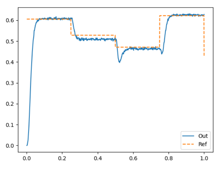
Here’s an example output of a network computing the STD on random 10-dimensional vectors:

Here’s the code I used to generate that figure:
test_nengo_std.py (1.5 KB)

You’ll notice that it does a reasonably good job computing the STD function, but it can at times be fairly incorrect. This is because the square root function is somewhat difficult to represent correctly, so you’ll need to play with the parameters of the mean_of_sqr ensemble. Here’s a test square root network you can use to do this:
test_nengo_sqrt.py (755 Bytes)

I should note that none of this code involves PES learning at all, and you must decide how you want to incorporate learning into these networks. With PES learning, you need to generate an error signal, which in turn requires a “reference” value (i.e., something that computes the function perfectly already), and I’m not quite sure how you want to do this. This Nengo example demonstrates this point.

1 Like

Hi, @xchoo , :blush:

Thanks for answering my questions in such detail. Your statements about neural networks in Nengo were of total importance for a better understanding of what I have been looking for in my research. This last implemented code, intuitively represents what in practical terms I want to do.

I really want to create a network to extract features or attributes from a discrete electrocardiogram signal, using supervised learning (PES). The solution presented by you was an interesting collaboration to better understand my problem (I’m new to Nengo and I still have some difficulties to express myself…)

I thank you in advance for your cooperation in my research.