Implementing Regression Model

I am tring to implement a regression problem which I will eventually implement on Loihi. I started with the MNIST classification problem example and tried to modify the compile section.

I replaced the RMSprop(0.001), SparseCategoricalCrossentropy, and sparse_categorical_accuracy with
Adam(0.001), MeanSquaredError, and Accuracy (as I used in Neural network model)

Unfortunately I am getting 0% accuracy unless I convert it as classification problem

Input: 4 x 3 and Output: 1 x 3

My code is attached below:

import warnings                 
import matplotlib.pyplot as plt
import nengo
import nengo_dl
import nengo_loihi
import numpy as np
import tensorflow as tf
from tensorflow.keras.models import Sequential, clone_model
from tensorflow.keras.layers import Input,Dense, Dropout, Activation, Flatten,Conv2D
from tensorflow.keras.layers import MaxPooling2D
from tensorflow.keras.datasets import mnist
from tensorflow.keras.utils import normalize
from urllib.request import urlretrieve
import pickle

# ignore NengoDL warning about no GPU
warnings.filterwarnings("ignore", message="No GPU", module="nengo_dl")
np.random.seed(0)
tf.random.set_seed(0)
num_classes = 3
# load dataset 
train_X= np.array([[[ 0.,  0.,  1.],
                    [ 0.,  1.,  1.],
                    [ 0.,  2.,  1.],
                    [ 1., -1.,  0.]],
                   [[ 0.,  0.,  1.],
                    [ 0.,  1.,  1.],
                    [ 0.,  2.,  1.],
                    [ 2., -1.,  0.]],
                   [[ 0.,  0.,  1.],
                    [ 0.,  1.,  1.],
                    [ 0.,  2.,  1.],
                    [ 3., -1.,  0.]]])
train_Y = np.array([[0.029, 0.059, 0.079],
                    [0.298, 0.985, 0.546],
                    [0.854, 0.911, 0.405]])
# Label modification like Mnist  
labels = []
for i in range(train_Y.shape[0]):
    output = np.argmax(train_Y[i])
    labels.append(int(output))
labels = np.array(labels)
train_images_R = train_X.reshape((train_X.shape[0],train_X.shape[1]*train_X.shape[2])) #NO need
train_labels_R = train_Y.copy() #NO need
train_Images = train_X.reshape((train_X.shape[0], 1, -1))  # 3,4,3 => 25,1,12 
train_Labels = train_Y.reshape((train_Y.shape[0], 1, -1))  # 3,3 => 3,1,3
train_Labels_RM = labels.reshape((labels.shape[0], 1, -1)) # 3, => 3,1,1 

def modelDef():
    inp = tf.keras.Input(shape=(4, 3, 1), name="input")
    # transform input signal to spikes using trainable 1x1 convolutional layer
    to_spikes_layer = tf.keras.layers.Conv2D(
        filters=3,  # 3 neurons per pixel
        kernel_size=1,
        strides=1,
        activation=tf.nn.relu,
        use_bias=False,
        name="to-spikes",
    )
    to_spikes = to_spikes_layer(inp)
    # on-chip layers
    flatten = tf.keras.layers.Flatten(name="flatten")(to_spikes)
    dense0_layer = tf.keras.layers.Dense(units=10, activation=tf.nn.relu, name="dense0")
    dense0 = dense0_layer(flatten)
    # since this final output layer has no activation function,
    # it will be converted to a `nengo.Node` and run off-chip
    dense1 = tf.keras.layers.Dense(units=num_classes, name="dense1")(dense0)
    
    model = tf.keras.Model(inputs=inp, outputs=dense1)
    model.summary()
    return model
    
def train(params_file="./keras_to_loihi_params123", epochs=1, **kwargs):
    model = modelDef() 
    miniBatch = 3
    converter = nengo_dl.Converter(model, **kwargs)

    with nengo_dl.Simulator(converter.net, seed=0, minibatch_size=miniBatch) as sim:        
        '''
        Followed MNIST classification structure
        '''
        # sim.compile(
        #     optimizer=tf.optimizers.RMSprop(0.001),
        #     loss= {
        #         converter.outputs[model.get_layer('dense1')]: tf.losses.SparseCategoricalCrossentropy(
        #               from_logits=True
        #           )
        #       },
        #     metrics={converter.outputs[model.get_layer('dense1')]: tf.metrics.sparse_categorical_accuracy},
        #     )
        # sim.fit(
        #     {converter.inputs[model.get_layer('input')]: train_Images},
        #     {converter.outputs[model.get_layer('dense1')]: train_Labels_RM},
        #     epochs=epochs,
        # )
        '''
        Not followed MNIST structure
        '''
        sim.compile(
            optimizer=tf.optimizers.Adam(0.001),
            loss= {
                converter.outputs[model.get_layer('dense1')]: tf.losses.MeanSquaredError()
                },
            metrics={converter.outputs[model.get_layer('dense1')]: tf.metrics.Accuracy()},
            )
        sim.fit(
            {converter.inputs[model.get_layer('input')]: train_Images},
            {converter.outputs[model.get_layer('dense1')]: train_Labels},
            epochs=epochs,
        )            
# train this network with normal ReLU neurons
train(
    epochs=2000,
    swap_activations={tf.nn.relu: nengo.RectifiedLinear()},
)

Could you please suggest me how to fix the issue (compile section)?

This is because accuracy only makes sense in the context of a classification problem. It compares how often your predictions equal your targets. Since you’re doing regression, your predictions will never be exactly equal to the targets.

I would recommend using tf.keras.metrics.MeanSquaredError() for your metric (or getting rid of the metrics entirely, since if you use MeanSquaredError, it will just be the same as your loss).

1 Like

Thanks for your suggestion. I trained the network, but it is not able to generate results accurately. During the training (epochs = 2000), the model converged (loss = 0).

Epoch 999/1000
3/3 [==============================] - 0s 3ms/step - loss: 4.4954e-12 - probe_loss: 4.4954e-12 - probe_mean_squared_error: 4.4954e-12
Epoch 1000/1000
3/3 [==============================] - 0s 3ms/step - loss: 4.7453e-12 - probe_loss: 4.7453e-12 - probe_mean_squared_error: 4.7453e-12

But when I tested the model, it could not generate desired results even with the trained data. For the first sample, model generated outputs are

Predict Outcome is: [[0.18543294 0.59750223 0.35057712]]
Actual Outcome is:  [[0.029 0.059 0.079]]

Code used for the testing is shown below. I also run the test on loihi cloud.

run_network(
    activation=nengo.SpikingRectifiedLinear(),
    scale_firing_rates=100,
    synapse=0.005,)
run_network(
    activation=nengo_loihi.neurons.LoihiSpikingRectifiedLinear(),
    scale_firing_rates=100,
    synapse=0.005,
)
run_network_onLoihi()

    def run_network(
        activation,
        params_file="./keras_to_loihi_params123",
        n_steps=30,
        scale_firing_rates=1,
        synapse=None,
        n_test=10, # only predict one sample, so no need of it.
        # test image, minibatch
    ):
        model = modelDefSmall_2()
        sample = 0 # temporary use for test sample creation
        # convert the keras model to a nengo network
        nengo_converter = nengo_dl.Converter(
            model,
            swap_activations={tf.nn.relu: activation},
            scale_firing_rates=scale_firing_rates,
            synapse=synapse,
        )
        # get input/output objects
        nengo_input = nengo_converter.inputs[model.get_layer('input')]
        nengo_output = nengo_converter.outputs[model.get_layer('dense1')]
        
        # test tiled input (for prediction)
        test_inputs = train_Images[sample]
        tiled_test_images = np.tile(test_inputs, (1, n_steps, 1))
        # set some options to speed up simulation
        with nengo_converter.net:
            nengo_dl.configure_settings(stateful=False)
    		
        # build network, load in trained weights, run inference on test images
        with nengo_dl.Simulator(
            nengo_converter.net, minibatch_size=1, progress_bar=False
        ) as nengo_sim:
            nengo_sim.load_params(params_file) 
            data = nengo_sim.predict({nengo_input: tiled_test_images})

        # compute accuracy on test data, using output of network on
        # last timestep
        predictions = data[nengo_output][:, -1]
        print("Predict Outcome is: {}".format(predictions))
        #predictions_max = np.argmax(data[nengo_output][:, -1], axis=-1)
        predictions_max = np.argmax(predictions)
        print("Predict Label is: {}".format(predictions_max))
        #print("Actual Label is:  {}".format(train_Labels[:n_test, 0, 0]))
        print("Actual Outcome is:  {}".format(train_Labels[sample]))
        print("Actual Label is:  {}".format(np.argmax(train_Labels[sample])))

Can anyone suggest ( or sample example) how to improve the accuracy in regression-based implementation? The model shows converging results during training but not able to generate accurate results during testing.

Hi @nayimrahman,

As @Eric suggested, you should:

If you have that working, and it seems like using the mean squared error does improve the training loss, then the issue might be something else. It’s hard to debug deep learning models without knowing the full details of the mode and the dataset characteristics, and even then, trying to figure out what is wrong with a DL model is a little bit of a black art.

Generally, when trying to debug models, you’d want to remove as much complexity from the system first, getting that to work, and then start slowly adding complexity in. In this case, since your model is a Keras model, I’d recommend first testing to see if the training and prediction gives satisfactory results in TensorFlow. Once you get it to train and predict will in TensorFlow, then start experimenting NengoDL, but don’t use spiking neurons yet. Stick with the rate-based ReLu neurons until you get decent performance, then move on to the spiking neurons.

Using this method of debugging, you’ll at least get a sense of what exactly is causing the performance issues with your model. :slight_smile:

1 Like

I followed your code but I got this error

AttributeError: type object 'function' has no attribute 'from_config' from converter = nengo_dl.Converter(modelDef, **kwargs)

train  (8672, 1, 17),  test (964, 1, 17), train labels((8672, 1, 1) and test labels (964, 1, 1)
def modelDef():
  inp = tf.keras.Input(shape=(1,8672,1,), name="input")
  to_spikes_layer = tf.keras.layers.Conv2D(

          filters=3,  # 3 neurons per pixel
          kernel_size=1,
          strides=1,
          activation=tf.nn.relu,
          use_bias=False,
          name="to-spikes",
      )

  to_spikes = to_spikes_layer(inp)
  flatten = tf.keras.layers.Flatten(name="flatten")(to_spikes)
  dense0_layer = tf.keras.layers.Dense(units=10, activation=tf.nn.relu, name="dense0")
  dense0 = dense0_layer(flatten)
  # since this final output layer has no activation function,
  # it will be converted to a `nengo.Node` and run off-chip
  dense1 = tf.keras.layers.Dense(units=num_classes, name="dense1")(dense0)

  model = tf.keras.Model(inputs=inp, outputs=dense1)
  model.summary()

  return model

def train(params_file="./keras_to_loihi_params", epochs=1, **kwargs):
    converter = nengo_dl.Converter(modelDef, **kwargs)
    with nengo_dl.Simulator(converter.net, seed=0, minibatch_size=200) as sim:
        sim.compile(
            optimizer=tf.optimizers.RMSprop(0.001),
            loss={
                converter.outputs[dense1]: tf.losses.SparseCategoricalCrossentropy(
                    from_logits=True
                )
            },
            metrics={converter.outputs[dense1]: tf.metrics.sparse_categorical_accuracy},
        )
        sim.fit(
            {converter.inputs[inp]: train},
            {converter.outputs[dense1]: train_Labels},
            epochs=epochs,
        )
        # save the parameters to file
        sim.save_params(params_file)

train(
    epochs=2,
    swap_activations={tf.nn.relu: nengo.RectifiedLinear()},
)

Hi @ssp ,

There doesn’t seem anything wrong in that particular part of the code that you attached, so I would assume that the error originates from some other part of the code. Unfortunately, without the full code to run, I will be unable to speculate as to the exact cause of this error. If you could post the script, or jupyter notebook, or a minimal version of the code that exhibits this behaviour, that would be much more helpful.

I have attached the code. PFA
I want to do the regression task. I built the model but when I tried to simulate using

# Train with NengoDL simulator
with nengo_dl.Simulator(net, minibatch_size=100) as sim:
    
    sim.compile(loss={out_p_filt: classification_accuracy})
print(
    "Accuracy after training:",
    sim.evaluate(test_images, verbose=0)["loss"],
)

But I got this errortest_simulation.py (4.6 KB) SimulatorClosed: Cannot call evaluate after simulator is closed

Hello, @xchoo thanks for responding.
I simulated this code again, now it worked after changing the loss and training dimensions But I am bit confused on “how to interpret these results?”
I predicted the muscle activities for 8 different targets but in general could you guide me on how to interpret it ?


MSE Nengo run net prediction of 1200 samples: 3.9005853530684655

Without knowing what data you used for the model, or what you are probing from the model, or how you intend to interpret the probed data, it is hard for an outsider to interpret these results. Typically, it is up to the principal investigator (i.e., the person who is using the model to address some problem) to figure out what data to use, and what model architecture to use, and to have a hypothesis as to the behaviour behind the model (e.g., "layer 1 is a feature detector, so we should see feature like filters there).

Since I do not have any of that background information, I cannot do much to interpret these results other than saying that the probed output appears to be rather spiky. To that, I’d refer you to this NengoDL example that goes through how to convert a Keras model into a spiking network, and how to configure the NengoDL converter to smooth out the spiky data. I’d also recommend not using a spiking network until you are clear as to what your network is supposed to do. The additional spikes may just serve to confuse the interpretation of the probed data.

Thanks for responding. Now I am able to interpret.
I have a quick question on “how to extract intermediate or any of the hidden layer output from an SNN?”
Moreover I want to compare how the neurons are activated in the Keras model and converted-SNN models for regression tasks.

convert the keras model to a nengo network

nengo_converter = nengo_dl.Converter(
    model,
    swap_activations={tf.nn.relu: activation},
    scale_firing_rates=scale_firing_rates,
    synapse=synapse,
)

inputLayer = model.get_layer('input_1')
hiddenLayer1 = model.get_layer('dense_1')
outputLayer = model.get_layer('dense_2')

 # get input/output objects
nengo_input = nengo_converter.inputs[inputLayer]
nengo_output = nengo_converter.outputs[outputLayer]

Hello @ssp,

Before simulating your Spiking network, you can create Nengo probes to your spiking layers (i.e. Conv/Dense with SpikingRectifiedLinear()) as follows:

 with nengo_converter.net:
        conv0_probe = nengo.Probe(nengo_converter.layers[conv0][sample_neurons])

where sample_neurons is an array of neuron indices which you want to probe (it’s a small hack to save memory as well by probing for smaller number of neurons, other wise conv0_probe = nengo.Probe(nengo_converter.layers[conv0] also works well!). conv0 is of course your TF Conv tensor object.

Then after simulating your SNN, you can get the spikes as:
scaled_data = data[conv0_probe][ii] * scale_firing_rates * dt # where dt = 0.001 and then plot it using rasterplot (i.e. from nengo.utils.matplotlib import rasterplot). It takes timesteps array in milliseconds e.g. [0.001, 0.002, 0.003, …] and spikes matrix in shape (timesteps, num_neurons).

I am linking two sources which can help you further. Here you will find how to get spikes (in cell [6]) and here an easy way to plot them.

Thanks for responding,
I tried to create nengo_probes could you please check it once?

This is my network so far,

steps = 30

inTrainNgo = np.tile(X_train[:, None, :], (1, steps, 1))

outTrainNgo = np.tile(Y_train[:, None, :], (1, steps, 1))

inputValidationNgo = np.tile(X_test[:, None, :], (1, steps, 1))

outputValidationNgo = np.tile(Y_test[:, None, :], (1, steps, 1))

inputTestNgo = np.tile(X_test[:, None, :], (1, steps, 1))

outputTestNgo = np.tile(Y_test[:, None, :], (1, steps, 1))

print(outputValidationNgo.shape)

input = tf.keras.Input(shape=(17,))

x1 = tf.keras.layers.Dense(50,activation=tf.nn.relu)(input)

x2 = tf.keras.layers.Dense(50,activation=tf.nn.relu)(x1)

output = tf.keras.layers.Dense(47,activation=tf.nn.relu)(x2)

model = tf.keras.Model(inputs=input, outputs=output)

model.summary()

converter = nengo_dl.Converter(

model,

swap_activations={tf.nn.relu: nengo.RectifiedLinear()},

)

net = converter.net

nengo_input = converter.inputs[input]

nengo_output = converter.outputs[output]

nengo_prob1 = converter.layers[x1]

with converter.net:

  •    conv0_probe = nengo.Probe(converter.layers[x1])*
    

run training

with nengo_dl.Simulator(net, minibatch_size=100, seed=0) as sim:

net.config[nengo.Ensemble].max_rates = nengo.dists.Choice([100])

net.config[nengo.Ensemble].intercepts = nengo.dists.Choice([0])

net.config[nengo.Connection].synapse = None

neuron_type = nengo.LIF(amplitude=0.01)


sim.compile(

    optimizer=tf.optimizers.SGD(),

    loss={nengo_output: tf.losses.mse},

)

sim.fit(

    inTrainNgo, {nengo_output: outTrainNgo},

    validation_data=(inputValidationNgo, outputValidationNgo),

    epochs=50,

)

sim.save_params("./nengo-model-relu-lif_trial")     

return model,inputTestNgo

You are creating probes at two places for the same layer. Not sure if creating a probe (i.e. nengo_prob1) outside the converter.net scope will work. Moreover you are using nengo.RectifiedLinear() in swap_activations={tf.nn.relu: nengo.RectifiedLinear()}, which isn’t a spiking neuron, hence you won’t see any spikes. I would suggest you to run your code and try plotting the spikes. In case you incur issues, let us know with the error message!

Thanks, sir for responding. I have fixed that but not sure how to do a raster or curved plot for all activation,

this is my plot code,

plot the results

for ii in range(3):

    plt.figure(figsize=(30, 8)

    plt.subplot(1, 3, 1)

    scaled_data = data[probe_l1][ii] * scale_firing_rates

    print(scaled_data)

    if isinstance(activation, nengo.SpikingRectifiedLinear):

        scaled_data *= 0.001

        rates = np.sum(scaled_data, axis=0) / (n_steps * nengo_sim.dt)

        plt.ylabel("Number of spikes")

    else:

        rates = scaled_data

        plt.ylabel("Firing rates (Hz)")

    plt.xlabel("Timestep")

    plt.title(

        "Neural activities (conv0 mean=%dHz max=%dHz)" % (rates.mean(), rates.max())

    )

    plt.plot(scaled_data)

    plt.subplot(1, 3, 2)

    plt.title("Output predictions")

    plt.plot(tf.nn.softmax(data[nengo_output][ii]))

    #plt.legend([str(j) for j in range(48)], loc="upper left")

    plt.xlabel("Timestep")

    plt.ylabel("Probability")

    plt.tight_layout()

I am no Sir (not yet knighted! :joy:
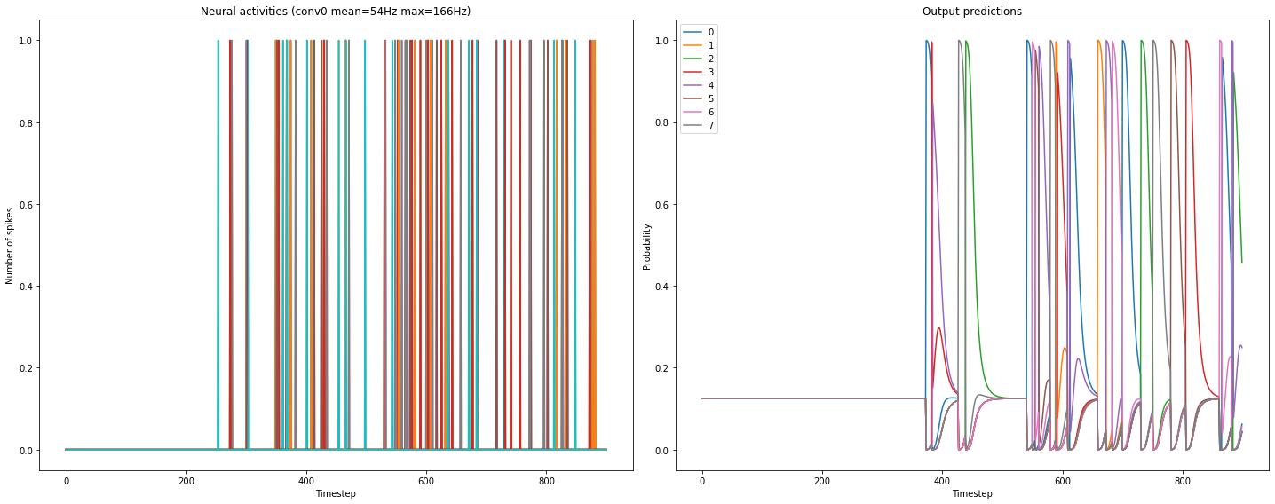
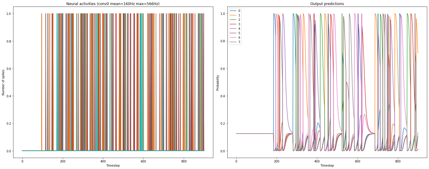
). With respect to plotting the spikes, I would suggest you to go step by step, and try to understand how spikes are calculated/represented.

As I mentioned in my previous reply,

scaled_data = data[conv0_probe][ii] * scale_firing_rates * dt # where dt = 0.001

gives you the spikes where data is the output of sim.predict(). In your above plotting code, scaled_data = data[probe_l1][ii] * scale_firing_rates doesn’t give you spikes yet, you still need to multiply by the dt (which is 0.001 in your case, unless you changed it during simulation). This is done in scaled_data *= 0.001 line. This line rates = np.sum(scaled_data, axis=0) / (n_steps * nengo_sim.dt) calculates the firing rate from the spikes scaled_data. Once you would simply print scaled_data, it should like [0, 0, 10.0, 0, 0, 10.0, 0, 0, 10.0 ...], i.e. a bunch of zeros and non-zero values. The non-zero values are the spikes (more accurately → spike amplitudes).

Now, it should be very easy to plot it, a simple plt.plot(scaled_data) should show you where (and how) the spikes occur - the plotting curve will be continuous though. Therefore, for aesthetic reasons, we plot it via a rasterplot(), to get discrete lines in place of spikes.

For using rasterplot(), as I mentioned in my previous reply, reshape scaled_data (if not already in) your neuron spikes matrix as (timesteps, num_neurons). That is, if you are simulating your network for 40ms, and trying to plot spikes for 3 randomly selected neurons, your scaled_data (before feeding to rasterplot()) should look like: (40, 3) matrix, i.e. each column corresponds to a neuron, and it has the temporal spikes along the row axis. Another argument to your rasterplot() should be timesteps themselves, i.e. timesteps = np.arange(sim_tsteps) * dt. Therefore the function call should be rasterplot(timestep, scaled_data). If you don’t want to use rasterplot(), you can refer the def plot_spikes() function in this tutorial as well.

Overall, you may be required to first understand the linked tutorials line by line, see the outputs of the spike matrices, etc. before learning how to plot them.

Thank you so much for the detailed explanation. It really helped a lot.
But I have another dumb question,
I am following this example, when the model Is predicting 2 let’s say, at that point, the plots shows the timestep from 0 to 9, in that case how to extract the neurons which predicted 2 or 3 ?
https://www.nengo.ai/nengo-dl/examples/keras-to-snn.html

I have extracted the scaled_data, which has 100 neurons based on my model but now I am confused on how to find which neurons predicted particular target?

Hello @ssp, I am not entirely sure of your question. But, in case you intend to look at the dynamics of the neuron which predict a particular number, then here’s my suggestion. The last Dense layer has the neurons which are responsible for predicting the probability scores of each digit (from 0 to 9 of course). Here’s the code which calculates the probability scores from the logits: tf.nn.softmax(data[nengo_output][ii]). You will find it in the run_network() in the same link you mentioned above.

Thus, in the linked tutorial case, the last Dense layer has 10 neurons (each neuron corresponding to a digit), and you just need to monitor them, e.g. the 3rd neuron upon monitoring will show if the neuron thinks the input image is that of 2 or not, the 10th neuron will show if it thinks that the input image is that of 9 or not… and so on. You just need to set a Probe to the last Dense layer and then you can monitor the output neurons’ behaviour throughout all the simulation timesteps.

However, in case you are planning to scan all the neurons in the network and then identify which neurons (in different layers) got activated (or are responsible for predicting) when input image of 2 was shown, it’s going to be very difficult manual task I suppose.

Sorry to bother you again.
I extracted the neurons from a Keras-sequential model using these command and then checked which neurons are max activated. Similarly in SNNs, can we extract the neurons associated within hidden layers ? or which neurons are max activated for targets?

get_1st_layer_output = K.function([model.layers[0].input],
                                  [model.layers[1].output])
layer_output = get_1st_layer_output([X])

Unfortunately I am unable to understand your linked code. However, going with the basics, you can certainly check which spiking neurons in SNNs (in any layer) have activated the most.

In TF-Keras models, there is no temporal dimension while training/inference. Thus, you can simply probe the non-spiking neurons, may be plot the activation maps / heat maps based on their probes output, or do some sort of calculation on their activation values to determine if they are max activated. Since I haven’t done this ever, I am also not sure if there exists a function in TF to help you with it. If at all there exists such a function in TF and you are looking for its equivalent in NengoDL, then I am afraid, it seems there isn’t any.

Although, you can do some basic maths with spiking neurons probed outputs to find which ones are max activated. First, you of course need to probe the spiking neurons of the layers you are interested in, then get their spikes, and then calculate their firing rate which has been done in the tutorial you are referring to. The firing rates of the spiking neurons closely correspond to their activation values in TF environment, i.e. they will be correlated. Thus, you can check which spiking neurons are max activated.

Or, there’s another easy method if you are not interested in explicitly calculating the spikes. You can simply probe the synapsed output of the spiking neurons (for the last timestep of your simulation), and that will give you it’s “oscillating” activation value (it will be oscillating due to spiking behaviour), and that will generally give you a good approximation of the actual activation value had the model been run in TF environment (you will find the TF activation values and NengoDL activation values to be correlated).

To probe only for the last timestep, you can set the following setting:

with ndl_model.net:
  nengo_dl.configure_settings(keep_history=False)

where ndl_model = nengo_dl.Converter(model). This will save enormous amount of memory. You can get more info about it here. To probe synapsed values from a layer, you can refer the following example:

with nengo_converter.net:
        conv0_probe = nengo.Probe(
                nengo_converter.layers[conv0][sample_neurons], synapse=0.005)

Just that it’s going to be a bit of long grunt work, so you have to be careful while coding. For crosschecking if your code is all right, you may plot the correlation plot of non-spiking neurons activation values (obtained in TF environment) and spiking neurons last timestep activation values (obtained in NengoDL environment). The scatter (correlation) plot for randomly chosen neurons (same for both the environments) for Conv/Dense layers would look like the following: