This is a somewhat unconventional way of representing visual input in a neural network. Normally you would want to play to the strengths of neural representation and encode a larger image using heterogeneous neurons and a distributed representation – see Encoding for image recognition for a few examples, or this spiking MNIST deep learning example.
You can do this if it’s what you want to be doing. You would supply the array as direct input current to a group of 25 neurons, and then probe their spiking activity, like so:
import nengo
import numpy as np
import matplotlib.pyplot as plt
one = np.asarray([
0,0,1,0,0,
0,0,1,0,0,
0,0,1,0,0,
0,0,1,0,0,
0,0,1,0,0,
])
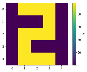
two = np.asarray([
0,1,1,1,0,
0,0,0,1,0,
0,1,1,1,0,
0,1,0,0,0,
0,1,1,1,0,
])
n_neurons = 25 # 5 times 5
freq = 100 # firing rate when input is 1
tau_stim = 0.005 # time-constant on stim -> vision
tau_probe = 0.1 # time-constant on vision probe
with nengo.Network() as model:
stim = nengo.Node(output=two)
vision = nengo.Ensemble(n_neurons=n_neurons, dimensions=1,
max_rates=freq * np.ones(n_neurons),
intercepts=np.zeros(n_neurons))
nengo.Connection(stim, vision.neurons, synapse=tau_stim)
probe = nengo.Probe(vision.neurons, synapse=tau_probe)
with nengo.Simulator(model) as sim:
sim.run(1.0) # run for 1 second
last_output = sim.data[probe][-1]
plt.figure()
plt.imshow(last_output.reshape((5, 5)))
plt.colorbar(label='Hz')
plt.show()
Visualizing the filtered spike-trains after 1 second of simulation: