Generating highly similar SPA vectors

I’m trying to generate highly similar vectors in SPA. This method, wherein I add a random vector to a previous vector, works:

import nengo.spa as spa

D = 16
n_items = 3

vocab = spa.Vocabulary(D)
S1 = vocab.parse('S1')

for i in range(2, n_items+1):
    v = vocab.parse('S1+0.4*R%d' % (i-1))
    v.normalize()
    vocab.add('S%d' % i, v)

print(np.dot(vocab.parse('S1').v, vocab.parse('S2').v))
print(np.dot(vocab.parse('S1').v, vocab.parse('S3').v))
print(np.dot(vocab.parse('S2').v, vocab.parse('S3').v))

Which gives:

0.921331459436
0.924898451434
0.755953671291

However, this other method doesn’t, despite essentially doing the same thing:

input_similarity = 1
vocab = spa.Vocabulary(D)

base = vocab.create_pointer()
vocab.add('X0', base)

for i in range(1, n_items):
    v = base + input_similarity * vocab.create_pointer()
    v.normalize()
    print(np.dot(base.v, v.v))
    vocab.add('X%d' % i, v)

Which gives:

0.618859679553
0.5922052248

What’s an easy way to generate SPA vectors within a similarity of each other?

The input_similarity in your second example is 1 (the equivalent factor in the first example is 0.4) which makes me think that the results are actually expected.

Alternative method of generating a set of vectors with known similarity: Define a symmetric similarity matrix target_cor, factorize it, and project it into a high-dimensional space. Example:

n = 6  # number of position vectors
indices = np.arange(n, dtype=int)
x, y = np.meshgrid(indices, indices)
target_cor = np.exp(-np.abs(x - y))
# Let's make the example a bit more complicated
target_cor[1, 3] = target_cor[3, 1] = -0.2
target_cor[0, 5] = target_cor[5, 0] = 0.6

u, s, v = np.linalg.svd(target_cor)

assert np.allclose(u, v.T)
assert np.allclose(np.linalg.norm(u, axis=1), 1)

base_pos_v = np.dot(u, np.diag(np.sqrt(s)))
assert np.allclose(np.linalg.norm(base_pos_v, axis=1), 1)

d = 128
up_proj = np.dot(np.random.permutation(np.eye(d)[:, :n]), base_pos_v.T)
1 Like

In this example, I understand that my target similarity is defined in the line target_cor[0, 5] = target_cor[5, 0] = 0.6, but how is target_cor[1, 3] = target_cor[3, 1] = -0.2 determined? I ask, because when I set target_cor[0, 5] = target_cor[5, 0] = 0.9, assert np.allclose(np.linalg.norm(base_pos_v, axis=1), 1) starts to fail due to exceeding the tolerance slightly.

Those are just arbitrary values. There are, however, matrices for which the factorization is not possible (I believe). But in your case it might just be that the numerical tolerance for the assert is too tight.

After talking to Jan a bit, he explained that for my specific case, this code was sufficient:

n_items = 6  # number of position vectors
indices = np.arange(n_items, dtype=int)
target_cor = np.ones((n_items, n_items)) * 0.9
np.fill_diagonal(target_cor, 1.)

u, s, _ = np.linalg.svd(target_cor)

assert np.allclose(np.linalg.norm(u, axis=1), 1.)

base_pos_vec = np.dot(u, np.diag(np.sqrt(s)))
assert np.allclose(np.linalg.norm(base_pos_vec, axis=1), 1)

d = 128
up_proj = np.dot(np.random.permutation(np.eye(d)[:, :n_items]), base_pos_vec.T).T

Here is an alternative to Jan’s approach that should be statistically equivalent but may seem less magical / more intuitive, as it has been derived directly from the geometry of the problem.

sphere = nengo.dists.UniformHypersphere(surface=True)

d = 3
b = 0.8  # desired similarity
u = sphere.sample(1, d=d)  # given vector

p = sphere.sample(1, d=d)
q = p - u.dot(p.T)*u
v = b*u + np.sqrt((1 - b**2) / q.dot(q.T))*q

print(u.dot(v.T))
print(v.dot(v.T))

Output:

[[ 0.8]]
[[ 1.]]

For some initial context, it may be helpful to orient yourself with the Gram–Schmidt process, as your problem can be almost viewed as a special case.

The intuition is to first recognize that if u is some d-dimensional vector on the surface of the hypersphere, then the vectors that have a dot-product with u of some fixed similarity b, will form a (d-1)-dimensional hyperplane with normal vector u. Moreover, this hyperplane cuts through the point b*u. Further constraining the required vector to be on the surface of the hypersphere amounts to restricting this hyperplane to be a hypersphere, that is, in essence, centered about the point b*u.

generating_similar

(Note that a 1-dimensional hypersphere is just the two end-points of a line segment. Three dimensions is where it becomes a bit more interesting, as the green vectors cut a circle from the dashed red hyperplane.)

Accordingly, we can first sample a point p on the surface (or ball, it doesn’t actually matter), and project (“squash”) it onto the hyperplane that is orthogonal to u. We can do this by just a single step of the Gram–Schmidt process, that is, by removing the part of p that is not orthogonal to u:

p = sphere.sample(1, d=d)
q = p - u.dot(p.T)*u

This just gives us a q such that u.dot(q.T) == 0. To see why (in case you don’t trust either Gram nor Schmidt), dot(u, q) == dot(u, p - dot(u, p)*u) == dot(u, p) - dot(u, p)*dot(u, u) == 0 since dot(u, u) == 1.

Now, to use this q, we just need to scale it by the appropriate constant (a) and add it to b*u so that its simultaneously on both the surface of the sphere and the aforementioned hyperplane. A quick picture along with Pythagorean’s theorem reveals that the scaling factor is a = np.sqrt((1 - b**2) / q.dot(q.T)) since the sides of the required right-angle triangle are a*q.dot(q.T) and b with a hypotenuse of 1.

And here is a visualization of this sampling procedure repeated 1000 times in 3 dimensions. The blue line is the given vector, u. The red dots are the q vectors (before normalization and shifting by b*u), and the green dots are the output (v) vectors. In each case, dot(u, v) == 0.8.

download

u = np.asarray([[1., 1., 1.]]) / np.sqrt(3)

from mpl_toolkits.mplot3d import Axes3D

plt.figure(figsize=(7, 7))
ax = plt.subplot(111, projection='3d')
ax.plot(*np.vstack((np.zeros(d), u)).T, c='b', lw=2) #*u.T, c='b')

for _ in range(1000):
    p = sphere.sample(1, d=d)
    q = p - u.dot(p.T)*u
    v = b*u + np.sqrt((1 - b**2) / q.dot(q.T))*q

    assert np.allclose(u.dot(v.T), b)
    assert np.allclose(v.dot(v.T), 1)
    
    ax.scatter(*v.T, c='g', alpha=0.5, s=2)
    ax.scatter(*q.T, c='r', alpha=0.5, s=3)
    
ax.set_xlim3d(-1, 1)
ax.set_ylim3d(-1, 1)
ax.set_zlim3d(-1, 1)
plt.show()
1 Like

This method only works if d > n, right?

Thanks for the awesome explanation and visualization.

I think I might have posed the problem incorrectly. If I understand correctly, this generates vectors similar to a base vector by a certain amount. I was hoping to generate N vectors whose pairs were all of the same similarity within a tolerance. Even with your explanation, I can’t imagine what this looks like on a hypersphere…

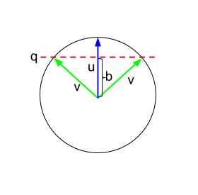
Ah! Well… it just so happens that you can also iterate the above procedure. In fact, this works out to be like an extended version of the Gram–Schmidt process! The trick is to maintain one matrix of orthogonalized vectors (via Gram–Schmidt), while simultaneously combining those vectors to build up the output matrix (via the above intuition). The challenge is to figure out the right scaling factors on these vectors in order to maintain the required invariant (by induction).

sphere = nengo.dists.UniformHypersphere(surface=True)

d = 6  # dimensionality
b = 0.8  # desired similarity

def proj(u, v):
    return u.dot(v.T) / u.dot(u.T) * u

M = np.zeros((d, d))       # output matrix
Q = np.zeros((d, d))       # Gram-Schmidt orthogonalization of S
S = sphere.sample(d, d=d)  # some random samples used to form Q

# Simultaneously apply Gram-Schmidt to S to compute Q while
# using Q to form M. This exploits the fact that
# Q[i, :].T.dot(M[j, :]) == 0 for all j < i.
for i in range(d):
    Q[i, :] = S[i, :]
    a = b/((i-1)*b + 1)
    for j in range(i):
        Q[i, :] -= proj(Q[j, :], S[i, :])
        M[i, :] += a*M[j, :]
    M[i, :] += np.sqrt((1 - i*a*b)/Q[i, :].T.dot(Q[i, :]))*Q[i, :]

print(M.dot(M.T))
[[ 1.   0.8  0.8  0.8  0.8  0.8]
 [ 0.8  1.   0.8  0.8  0.8  0.8]
 [ 0.8  0.8  1.   0.8  0.8  0.8]
 [ 0.8  0.8  0.8  1.   0.8  0.8]
 [ 0.8  0.8  0.8  0.8  1.   0.8]
 [ 0.8  0.8  0.8  0.8  0.8  1. ]]

I would derive the magic scaling constants, but LaTeX is currently broken here. There’s also a lot that can be said regarding the geometry of the problem to motivate this way of combining the vectors, but, for the time being, I will leave this as an exercise for the reader. [Hints: By way of induction, write down all known dot-products using what you know about Gram–Schmidt as well as the fact that each vector in M is a linear combination of vectors from Q.]

In the end, this should be equivalent to Jan’s approach, but gives a geometrical perspective that may seem less mysterious to some. Understanding Jan’s approach also has value (he has a notebook with some details here and there is some very related discussion here). Note that both approaches only work for n <= d (essentially by the rank-nullity theorem).

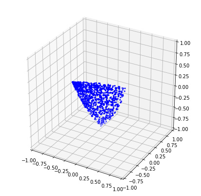
If we want n > d, then we require some sort of relaxation, for instance: bound the similarity below by some lower-bound. In this case, the d vectors of the matrix fully define the vertices of a convex surface from which to sample. More concretely, the surface is the set of all vectors on the sphere that have a dot-product of at least b with every vector in M. In this sense, the vectors in M act as “representatives” for the convex surface. Any two vectors drawn from this surface are guaranteed to have a similarity of at least b. Moreover, this surface has maximal area.

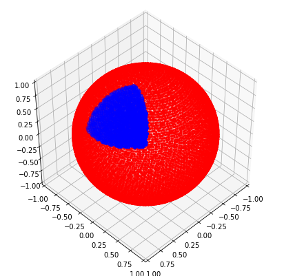
In three dimensions, this surface is an equilateral triangle covering the sphere. I haven’t tried thinking through a good way to uniformly sample this surface, apart from the obvious method of checking if random samples p satisfy np.all(M.dot(p.T) >= b) (see below).

download (1)

from nengolib.stats import sphere
from mpl_toolkits.mplot3d import Axes3D

good = []
bad = []
for p in sphere.sample(20000, d=d):
    if np.all(M.dot(p.T) >= b):
        good.append(p)
    else:
        bad.append(p)

good = np.asarray(good)
bad = np.asarray(bad)
assert np.all(good.dot(good.T) >= b)

plt.figure(figsize=(7, 7))
ax = plt.subplot(111, projection='3d')
ax.scatter(*bad.T, s=5, c='red')
ax.scatter(*good.T, s=20, c='blue')
#ax.scatter(*M.T, s=100, c='green')
ax.set_xlim3d(-1, 1)
ax.set_ylim3d(-1, 1)
ax.set_zlim3d(-1, 1)
ax.view_init(45, 45)
plt.show()

If you want to further restrict the dot-products to be no greater than some upper-bound, then things suddenly become much harder. In general, this reduces to the sphere-packing problem, which is an unsolved problem in mathematics. Only the solutions for a couple specific instances (e.g., the Leech lattice) are currently known. I would recommend randomly sampling, checking, and keeping/discarding (as done in the SPA).

One last thing worth mentioning: the above method assumes that the rows of S are linearly independent (in other words, they span the d-dimensional space). For uniformly and independently sampled vectors, this happens almost surely. However, with dependent sampling (e.g., nengolib.stats.sphere), this is no longer necessarily the case. So if you are experimenting with this, make sure that you are sampling/choosing S such that it can be orthogonalized, otherwise strange things may happen.

1 Like

Sorry didn’t realize this; should be fixed now.

For some reason, this approach isn’t working for higher dimensions, because it can’t find any good vectors.

from nengolib.stats import sphere
uniform_sphere = nengo.dists.UniformHypersphere(surface=True)

d = 16
b = 0.3

M = np.zeros((d, d))       # output matrix
Q = np.zeros((d, d))       # Gram-Schmidt orthogonalization of S
S = uniform_sphere.sample(d, d=d)  # some random samples used to form Q

for i in range(d):
    Q[i, :] = S[i, :]
    a = b/((i-1)*b + 1)
    for j in range(i):
        Q[i, :] -= proj(Q[j, :], S[i, :])
        M[i, :] += a*M[j, :]
    M[i, :] += np.sqrt((1 - i*a*b)/Q[i, :].T.dot(Q[i, :]))*Q[i, :]

good = []
bad = []
for p in sphere.sample(50000, d=d):
    if np.all(M.dot(p.T) >= b):
        good.append(p)
    else:
        bad.append(p)

print(len(bad))
assert len(good) > 0
good = np.asarray(good)
bad = np.asarray(bad)
assert np.all(good.dot(good.T) >= b)

The assert statement works for smaller dimensions, but not lower dimensions. This occurs regardless of me sampling uniform_sphere or sphere, so I’m guessing it doesn’t have to do whether the vectors are independently sampled or not? Also, I don’t think the problem is the number of samples either, unless I’m underestimating how small the similarity space is in higher dimensions.

Thanks!

Yes, you are underestimating how small.

For simplicity, let’s suppose b = 0 and imagine d is large (say 16 or greater). The convex surface described in my previous post is going to be the intersection of d half-planes, restricted to the sphere. Since the sphere is isomorphic under rotation, this is just one “quadrant” of the sphere after a change of reference coordinates. Stated simply: to randomly find a vector on this surface, we flip a coin d times, and it has to land heads every time. Thus, the probability is $\frac{1}{2^d}$.

Therefore, even for this generous case, we would expect to need 2**16 == 65536 (incidentally, this is only slightly larger than the 50000 you chose) samples before finding one in the valid region. For b > 0, this only becomes worse (less probable), as the region shrinks down in size.

In this case, you will probably want to sample the space a bit more carefully. You could probably use the vectors of M and Q, and an appropriately sampled linear combination, to do so, but I’m wary to make a concrete suggestion before thinking through whether it’s guaranteed to be uniform.

Disclaimer: This has not been tested for correctness, nor uniformity (I’m actually pretty sure that this is not uniform, and it is missing the rounded edges of the surface… but I guess it’s better than nothing if you are in a rush – it may still be better to combine the vectors in M and Q).

Here is a way of sampling this region using hyperspherical coordinates. I am just applying the above intuition (in regards to the convex surface) to uniformly sample spherical coordinates (angles), transforming them into Euclidean space, and then rotating the vectors by a random orthogonalization (in the same way as Jan’s approach, but you could also use Gram-Schmidt for the last step too).

b = 0.8  # desired minimum similarity
d = 16
num_samples = 1000

coords = np.random.uniform(size=(num_samples, d-1))*np.arccos(b)

s = np.sin(coords)
c = np.cos(coords)
mapped = np.ones((num_samples, d))
mapped[:, 1:] = np.cumprod(s, axis=1)
mapped[:, :-1] *= c

from nengolib.stats import random_orthogonal
good = mapped.dot(random_orthogonal(d))

assert good.shape == (num_samples, d)
assert np.allclose(np.linalg.norm(good, axis=1), 1)
assert np.all(good.dot(good.T) >= b)
print (np.min(good.dot(good.T)))

Output: 0.800504567559

Note that this code is almost identical to some code from nengolib.stats.spherical_transform.

And the following visualizes this for d = 3, b = 0.5.

download (2)

Rather than me continuing to rant on about things that may easily be misunderstood or seen as unimportant, feel free to ask questions here and I’ll explain more or attempt to extend this further.