Direct connections and postsynaptic potentials

Hi!

My project consists of translating a biologically detailed model of Basal Ganglia from NEST to Nengo. It is defined in terms of biological data (e.g. average number of connections from population A to population B, capacitance of A’s neurons, postsynaptic potentials…), not in terms of mathematical expressions. Therefore, I cannot really use NEF’s encoders and decoders. In this model, a command is represented by the activity of a discrete channel of neurons in ganglia. Once I implemented the model in Nengo using Direct Connections, will I be able to use it functionally (i.e. having inputs and outputs encodable and decodable by NEF)?

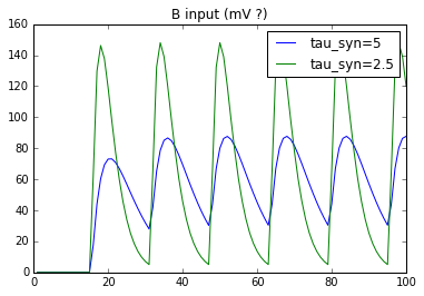
Moreover, I do not really understand how to choose the postsynaptic potential of a Direct Connection. In NEST, the following code creates a connection between population A and B that will cause postsynaptic potentials (PSP) of 1 mV in neurons of B. Amplitude of PSPs is therefore independent of synaptic time constants.

nest.SetStatus(A, {'tau_syn':[5.]}) # set synaptic time constant of receptor type 1
nest.Connect(A, B, syn_spec={'receptor_type':1, 'weight':1}) # connect A->B with weight (PSP) = 1

However, when I try to connect neurons of two populations in Nengo, the input of B seems to depend on the time constant of the synapse. I would expect the following code to exhibit the same behavior as NEST, with weights specified in the transform parameter:

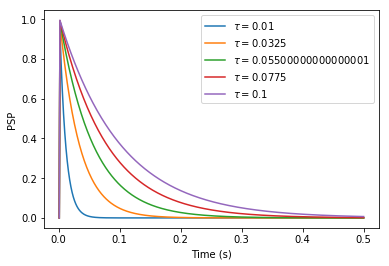
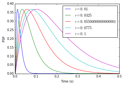
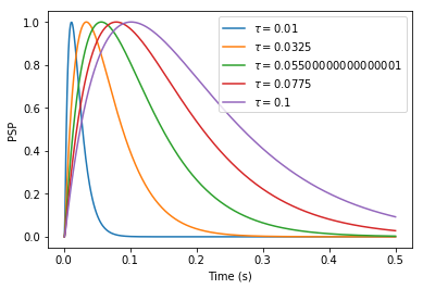
syn_AMPA = nengo.synapses.Alpha(tau_syn_AMPA/1000.)
nengo.Connection(A.neurons, B.neurons, transform=[1], synapse=syn_AMPA)

But when I probe the input of B, this is what I get:
t%C3%A9l%C3%A9chargement%20(1)

NB: transform does scale the input. But I would like to use it as an absolute value of PSP.

Can you please tell me how to properly set the weight/PSP of a direct connection and whether or not I will be able to encode/decode values?

You might be interested in looking at the nengo.networks.ActionSelection or the updated nengo_spa.modules.BasalGanglia for your own reference. There are some supporting papers and documentation too. Just FYI.

Interesting question. Normally we do one or the other, but there is nothing stopping you from using direct connections at the same time as having inputs encodable and outputs decodable. However, it might be difficult to do this in a way that is useful/interpretable. When you decode from an ensemble, you are projecting the activities down into a low-dimensional space that is some (possibly nonlinear) transformation of the space being encoded. So the decoding is always with respect to some encoding that you (as a modeller) define. By default this encoding is given by the uniformly distributed tuning curves and encoding vectors of some chosen dimensionality. When you use direct connections you are essentially bypassing this encoding (when connecting directly to neurons), or bypassing the decoding (when connecting directly from neurons). All this is to vaguely say: yes, but you just have to be aware of what this means, and decide whether it still makes sense for what you are trying to do.

In Nengo, the area under the PSP is held constant as you change the time-constant. The amplitude of the peak changes, but its integral is always 1. We do things this way because it ends up making things nice and consistent in a few ways. Mathematically this is implementing a convolution with the filter $h(t) = \frac{1}{\tau} e^{-t / \tau}$ which has an area of 1. If you are a control-theory person, this is “easy” to see by its Laplace transform, $H(s) = \frac{1}{\tau s + 1}$ since $H(0) = 1$. But I digress.

If you want to change the time-constant while keeping the amplitude of the peak constant, then you can take advantage of the fact that the height of the peak is proportional to $1 / \tau$. Thus, scaling the transform by $\tau$ will keep the peak the same, regardless of time-constant:

import numpy as np
import matplotlib.pyplot as plt
import nengo

spike = np.zeros(500)
spike[1] = 1 / 0.001  # 1/dt

plt.figure()
for tau in np.linspace(0.01, 0.1, 5):
    H = nengo.Lowpass(tau)
    plt.plot(H.ntrange(len(spike)), H.filt(spike * tau, y0=0), label=r"$\tau = %s$" % tau)
plt.xlabel("Time (s)")
plt.ylabel("PSP")
plt.legend()
plt.show()

PSPs
The important bit is to include a factor of tau in your transform (weights).

But be aware that now you’re also scaling the integral by $\tau$. And since downstream neurons essentially integrate their input currents, you will be indirectly scaling the total amount of current they get as well by the same factor, which in turn may scale up how often they spike. This is part of why our default behaviour is to keep the integral constant, since it keeps the total current constant.

1 Like

Thanks again for your perfect answer!

I already know about the implementation of [1] in Nengo. My goal is to implement a more biologically plausible model of humans’ BG which does not contain segregated pathways (unpublished spiking version of [2]). The aims of this project include:

  1. Assessing the functional performance of [2] with a naturalistic task (e.g. within the Tower of Hanoi architecture in Nengo or within Spaun)
  2. Study the impact of Parkinson’s disease (that can be simulated by [2]) on high-level cognition with such naturalistic tasks
  3. Evaluating how [2] performs in the task compared to [1] to assess the need for biological plausibility in cognitive modelling

[1] Gurney, K., Prescott, T., & Redgrave, P. (2001). A computational model of action selection in the basal
ganglia. Biological Cybernetics 84, 401-423.
[2] Liénard, J. & Girard, B. J Comput Neurosci (2014) 36: 445. https://doi.org/10.1007/s10827-013-0476-2

I really need to look more in depth into how NEF works because I think it can compromise my entire project… My goal is to use the implementation of [2] to perform action selection and compare with [1]. Hence I need to somehow figure out how to do encoding/decoding with the new model. But from my knowledge I cannot use regular Nengo connections as the model is defined with direct connections rather than mathematical transformations like [1]. Are you aware of other Nengo projects whose aim was to implement such a bottom-up defined model? Otherwise could you mention people who could know about similar projects here?

If I understand you correctly, that is exactly what I want. That is how NEST works (that’s what I can deduce from my simple experiments, one can correct me if I am wrong). The spiking version of [2] was implemented in NEST and I want to stick to every detail (until I face some limitation you cannot help me with :blush:).

It’s funny and interesting to see the difference between a bottom-up (NEST) and a functional (Nengo) spiking neuron simulator, as well as the tricks to translate one thing to the other.

Thanks again!

The BG network that I mentioned might be an instance of this, where it is defined bottom-up using direct connection weights, and the encoding/decoding is used to interface the action selection module with other cognitive modules that represent vectors (i.e., the semantic pointer architecture). I’m not sure if this is what you mean, or if you’re looking for ways to do this internally within the network as well. Either way, looping @tcstewar in on this as he has some better understanding and experience with people wanting to do such things!

@arvoelke your solution does not seem to work with nengo.synapses.Alpha():

image

Scaling the input by a factor of approximately 2.7189 seems to produce PSP of 1. However, the scaling factor still depends on tau. Can you please clarify this? Here is the code with the scaling factor:

import numpy as np
import matplotlib.pyplot as plt
import nengo

dt = 0.001
spike = np.zeros(500*1)
spike[1] = 1 / dt  # 1/dt

plt.figure()
for tau in np.linspace(0.01, 0.1, 5):
    H = nengo.synapses.Alpha(tau)
    plt.plot(H.ntrange(len(spike)), H.filt(spike * tau, dt = dt, y0=0)*2.7189, label=r"$\tau = %s$" % tau)
    print(np.max(H.filt(spike*tau, y0=0))*2.7189) #output depends on tau
plt.xlabel("Time (s)")
plt.ylabel("PSP")
plt.legend()
plt.show()

The alpha synapse will need a scaling factor of $\tau e$, where $e$ is Euler’s constant (np.e = 2.718...). Currently you have $\tau$ scaling the input, and an approximation of $e$ scaling the output – but, by linearity, you can multiply these two together.

To see where this comes from, the PSC (a.k.a., PSP) has the impulse response:

$$h(t) = \frac{t}{\tau^2} e^{-t/\tau}$$

This is given in the documentation (link). It can also be derived by considering the transfer function of two Lowpass(tau) multiplied together:

$$H(s) = \frac{1}{\left(\tau s + 1\right)^2}$$

and asking WolframAlpha for its inverse Laplace transform (link).

To find the peak of the impulse response, we differentiate with respect to $t$:

$$\frac{\partial h(t)}{\partial t} = \frac{\left( \tau - t \right)}{\tau^3} e^{-t/\tau}$$

Set this to $0$ and solve for $t$:

$$\frac{\partial h(t)}{\partial t} = 0 \iff t = \tau \text{ and } \tau \ne 0$$

And finally plug $t = \tau$ back into the impulse response:

$$h(\tau) = \frac{\tau}{\tau^2} e^{-\tau/\tau} = \frac{1}{\tau e}$$

For some extra validation, we can double-check all of this with WolframAlpha:

Therefore, since the peak of the alpha waveform is $\left(\tau e\right)^{-1}$, we must scale it by $\tau e$ to keep its peak fixed at $1$.

import numpy as np
import matplotlib.pyplot as plt
import nengo

spike = np.zeros(500)
spike[1] = 1 / 0.001  # 1/dt

plt.figure()
for tau in np.linspace(0.01, 0.1, 5):
    H = nengo.Alpha(tau)
    transform = tau * np.e
    plt.plot(H.ntrange(len(spike)), H.filt(spike * transform, y0=0), label=r"$\tau = %s$" % tau)
plt.xlabel("Time (s)")
plt.ylabel("PSP")
plt.legend()
plt.show()

alpha

I feel really bad for not recognizing Euler’s constant… Thanks :wink:

2 Likes