Hi, I am looking at this example in nengo_dl and I am confused about a few things in the 3rd cell:
with nengo.Network() as auto_net:
    # input
    nengo_a = nengo.Node(np.zeros(n_in))

    # first layer
    nengo_b = nengo.Ensemble(n_hidden, 1, neuron_type=nengo.RectifiedLinear())
    nengo.Connection(nengo_a, nengo_b.neurons, transform=nengo_dl.dists.Glorot())

    # second layer
    nengo_c = nengo.Ensemble(n_in, 1, neuron_type=nengo.RectifiedLinear())
    nengo.Connection(
        nengo_b.neurons, nengo_c.neurons, transform=nengo_dl.dists.Glorot()
    )

    # probes are used to collect data from the network
    p_c = nengo.Probe(nengo_c.neurons)
I was expecting the nengo_b = nengo.Ensemble(1000, n_hidden, neuron_type=nengo.RectifiedLinear()), since I thought the first parameter is number of neurons in the ensemble and second parameter is the dimensions in vector space representation. The example seems to initialize 64 neurons representing a scalar value. Is this correct?
Is there a reason why neuron_type=nengo.RectifiedLinear()? Will this still work if I changed neuron_type=nengo.LIF()?
Is there a reason why the connection is defined as nengo.Connection(nengo_a, nengo_b.neurons, transform=nengo_dl.dists.Glorot()) instead of nengo.Connection(nengo_a, nengo_b, transform=nengo_dl.dists.Glorot()) (connection to nengo_b ensemble as a whole)?
Why is the transform=nengo_dl.dists.Glorot()? I understand from deep learning that these are weight initialization functions, but doesn’t setting transform=nengo_dl.dists.Glorot() means that nengo_dl.dists.Glorot() is the function that is going to be represented by the decoders as described in NEF?
In that example, specifically for that cell, the goal was to replicate the TensorFlow network in the previous cell as a Nengo-native network. The TensorFlow network in question (from cell 2) is:
You are correct in the understanding that the first parameter is the number of neurons, and the second parameter is the dimensionality of the ensemble. However, neurons and layers (a.k.a., neural ensembles) in TensorFlow networks are typically initialized differently than in Nengo.
In Nengo, multi-dimensional information is represented in ensembles using the “dimension” argument. But this “dimension” is sort of an abstract consequence of the use of encoders and decoders (through the application of the NEF algorithm). In TensorFlow, however, it is typical to see 1 neuron used to represent 1 dimension. Hence, if a layer has an output “dimension” of 1000, it typically also means that the layer also has 1000 neurons.
Going back to the TensorFlow code, the layer is defined as such:
So, the dense layer has n_hidden number of neurons. Since TensorFlow doesn’t utilize the concept of individual neurons representing multiple dimensions, each neuron in the TensorFlow model is consider to represent a scalar value. Thus, the equivalent Nengo ensemble for that specific TensorFlow layer is:
In TensorFlow, neurons are typically initialized with the ReLU (rectified linear unit) activation function. In the reference TensorFlow code, it’s actually forced:
activation=tf.nn.relu
Thus, to match the TensorFlow model, the Nengo network is initialized with nengo.RectifiedLinear() neurons. Note that TensorFlow doesn’t (by default) support spiking neurons, so the neurons are nengo.RectifiedLinear as opposed to nengo.SpikingRectifiedLinear.
As to whether nengo.LIF would work? It should work, yes, but I expect the accuracy of the network to decrease when compared to the ReLU neurons. The ReLU neurons have a linear activation function (an increase in the input leads to a linearly proportional increase in the neuron’s output firing rate), which makes it easier for a single neuron to approximate complex functions (remember that in TensorFlow 1 neuron is mapped to 1 dimension of the output). LIF neurons, by contrast, have a non-linear activation function.
Yup.
In Nengo, when you make a connection to an ensemble object (as opposed to a .neurons object), Nengo treats this connection as having encoders & decoders. TensorFlow, however, doesn’t utilize the NEF algorithm (or even have the concept of the NEF built in it). Thus in TensorFlow, connections between layers don’t have encoders and decoders (they just have connection weights). To replicate this “lack of encoders & decoders” between the connections in Nengo, the connection is configured to connect to the .neurons object, rather than to the ensemble itself.
This is the reason why further down in the Nengo code, you’ll see this (connection from nengo_b.neurons to nengo_c.neurons:
There are two points of clarification here that I will address separately: about the use of transform and about the representation by decoders.
Use of transform
For Nengo connections, the transform parameter takes on multiple roles depending on what objects the connection connects to. In the context of connecting to a neuron object, whatever is specified in transform specifies the input weights to the neurons. When connecting from a neurons object, the transform specifies the output weights of the neurons. Thus, when making a neuron-to-neuron connection, transform specifies the full connection weight matrix between the two populations of neurons.
When creating connections to ensemble objects, however, the transform specifies a multiplication by some matrix (or scalar) on a decoded signal. When connecting to an ensemble, the connection will use the (post) ensemble’s encoders in the weight matrix, effectively making the neuron input weights T \times E (where T is the transform, and E are the encoders). When connecting from an ensemble, the connection will use the (pre) ensemble’s decoders, effectively making the neuron (post) output weights D \times T. When connecting two ensembles together, both the decoders (pre-ensemble) and encoders (post-ensemble) are used, and the full connection weight matrix is D \times T \times E.
Decoders
This part is just to clarify this statement you made:
This is not strictly the case. As I mentioned above, the transform is just a multiplicative factor on the weight matrix, and not the object used to define the ensemble’s decoders. Rather, the function parameter on nengo.Connections is the one used the solve for the ensemble’s decoders, and the transform is then rolled into the decoders as a multiplicative factor (by doing a matrix multiplication).
would give you the same decoders (for ens1) as this:
nengo.Connection(ens1, ens2, transform=2)
In the former code, Nengo will solve for the decoders that directly approximate the function f(x) = 2x. In the latter code, Nengo will solve for the decoders that approximate the function f(x) = x, and then apply the transform factor, which will scale up all of the decoders by a factor of 2, resulting in the same decoders from the former code.
It’s no problem! There definitely is a difference in the way “standard” machine learning treats neural networks and how the NEF treats them. So, confusion here is warranted.
Thanks @xchoo! This really cleared up a lot of my misunderstandings, especially on the differences between function=lambda x: 2*x and transform=2, and also the differences between nengo.Connection(a.neurons, b.neurons) and nengo.Connection(a, b).
I do have 1 clarification on whether the matrix multiplications mentioned above for transforms are elementwise multiplications?
The output activity of ens1 is represented as a 5D vector (one element representing the activity of each neuron): [a_1, a_2, ... , a_5]
The decoders of ens1, is a 5 x 2 matrix:
To obtain the input to ens2, we do \vec{x} \times T, and since \vec{x} is a 2D vector, and we want the input to ens2 to be a 3D vector, the transform matrix T has a shape (2, 3). So, we have:
where y_1 = x_1T_{11} + x_2T_{21}, and so forth for y_2 and y_3.
Note: In Nengo, the order of matrix operations is a little different (to keep consistent with the notation in the NEF book), so the transform matrix you provide is actually a transposed version of T above (see here, under the description for the transform parameter).
The input to ens2 then gets matrix multiplied with the encoders of ens2 to get the inputs(\vec{i}) to each neuron in ens2:
The inputs \vec{i} then get multiplied by the neuron gains, and added to the neuron biases, and fed through the neuron’s activation function to get the output activity of said neuron.
So, the full chain of matrix multiplications from output activity of ens1 to input to ens2 is:
From the math above, we see that we can combine a few matrices together to make the computation more efficient. For example, we can combine the decoders of ens1 and the transform matrix T together, just by doing one step of the matrix multiplication (i’m going to use A here for the notation for the matrix, but there isn’t really a set notation for this intermediate matrix):
Now, if you were to probe the connection’s weight matrix (i.e., doing sim.data[conn].weights), you’ll get the full connection weight matrix (once again, transposed from the math above).
I know it’s a lot of math in the post above, but I hope that clarifies things!
Hi @xchoo, the math is great! I now get a better picture of what is happening under the hood, but pardon me for wanting to really get to the bottom of this with more follow-up questions.
I am currently trying to build a “1-layer” autoencoder for MNIST data and learn the connection weights using PES learning rule. I reckoned that it should work since it is just 1 layer, but after implementing a part of it, I realized it may not be true:
with nengo.Network() as model:
    input = nengo.Node(size_out=784)
    hidden = nengo.Ensemble(n_neurons=500, dimensions=64)
    output = nengo.Ensemble(n_neurons=1000, dimensions=784)

    nengo.Connection(input, hidden, transform=?)
    conn = nengo.Connection(hidden, output, eval_points=X_train, function=X_train)
    conn.learning_rule_type = nengo.PES()

    error = nengo.Ensemble(n_neurons=1000, dimension=784)
    nengo.Connection(input, error, transform=-1)
    nengo.Connection(output, error)
    # Calculating MSE as the Error signal into conn.learning_rule
    nengo.Connection(error, conn.learning_rule, transform=lambda x: np.sum(np.square(x)))
I am stuck because this is not really a 1 layer neural network. There are actually 2 weight matrices to be learned, with 1 from the input to the hidden layer, and another from hidden layer to the output layer. As such I am not sure what to put for the transform=? in the first connection between input and hidden layer. I would like to ask if you have done something similar and how this issue can be overcome.
Another question that I have is whether the PES learning rule is updating the full weight connection matrix:
I seem to recall from somewhere that only the decoders are being changed, whereas the encoders, transform matrix remains static. I was wondering if there is some way I can update the transform matrix T, since it resembles the weight matrix of artificial neural networks.
There are several options here. You can leave it to the default value, in which case, a bunch of encoders will be randomly generated for the hidden ensemble. Or, you could set the input weights (either through transform or by setting the encoders) to some sort of filter to “pre-process” the MNIST digits. I recommend checking out this Nengo example which attempts to do something similar (classify an MNIST input in a single layer), but using the NEF solver rather than using the PES learning rule as you have in your code. (Note, you can find a list of other Nengo examples here!)
By default (and mathematically), the PES learning rule will only modify the decoders of the pre ensemble. However, you can modify the nengo.Connection syntax to have the PES learning rule apply the weight updates on the full connection weight matrix. To do this, you’ll need to provide a solver with the weights=True parameter when creating the nengo.Connection. An example:
When you give a solver (with weights=True) to a Nengo connection, it tells Nengo to create a connection between two ensembles but using the full connection weight matrix rather than by separating out the decoders, encoders, and everything else. Nengo does this by combining the decoders, encoders and any transformation matrices together to form the full connection weight matrix (see the math above).
When you apply the PES learning rule to these types of connections, the entire weight matrix is modified. However, it is important to note that mathematically, the PES updates are still doing the same thing. That is to say, even with a “full” connection weight matrix, only the decoders are being modified. It’s analogous to saying:
I have a number A = B \cdot C \cdot D
If I modify only B and keep C and D constant, A still changes
In the case of the full connection weight matrix, A is the full weight matrix, B are the decoders, C are the transform matrices, and D are the encoders. To understand how the PES learning rule accomplishes this, there’s a blurb about it in this Nengo example (see the part about “individual connection weights changes”).
I think I figured parts of it out by referring to the example and the math provided above. Given that I have three ensembles to represent an autoencoder:
the only way I can connect in_ensemble to hidden to out_ensemble without Nengo complaining about incompatible dimensions is to provide a matrix of size size_in x n_hidden and n_hidden x size_in as the transform matrix T. But since I also don’t want to just use any np.random.random((size_in, n_hidden)) matrix for my transform, I decided to create the matrix with Mask() and Gabor() instead:
# Encoders are used as transforms for dimension reduction
encoders = Mask(img_shape).populate(
    Gabor().generate(n_hidden, (11,11)),
    flatten=True
)
# Decoder transforms/weights for reconstruction
decoders = Mask(img_shape).populate(
    Gabor().generate(n_hidden, (11,11)),
    flatten=True
).T

conn1 = nengo.Connection(
    in_ensemble, hidden,
    transform=encoders
)
conn2 = nengo.Connection(
    hidden, out_ensemble,
    transform=decoders
)
Not sure if there are any undesirable effects if I use the Gabor filters this way, but it seems to resolve the dimension mismatch issue that I was stuck on earlier.
I do have some more questions regarding credit assignment of PES error signal to conn1 and conn2 now, but I am not sure if I should continue asking it in this thread since the discussion and the title is a bit different now.
I can’t say for certain what effect setting conn2’s transform to Gabor filters will have on the ability of the network to learn the desired function. In theory, because everything is a matrix multiplication (i.e., they are all linear transformations), it should matter what the value of transform is (be it Gabor filters, or random values), since the PES learning rule should be able to modify the decoders to compensate (or negate) whatever the initial transform on the connection was.
You can post those questions here, they will be related to your original question.
To pre-empt your questions, the PES learning rule is a local learning rule. That is to say that the learning rule typically uses an error signal that is locally generated (using the output of the ensemble, for example), and is used to modify only the weights in the connection (and no other connection).
For your problem in particular, I would focus first on only learning one connection (conn2 in particular). This way, you don’t have a credit assignment issue to deal with. If you do want to create a network where you are trying to learn two connections at the same time, you’ll want to have a clear idea of what function each of the connections is attempting to learn. I.e., we know that conn2 is meant to map the activities of hidden to some output vector (which for an autoencoder is clearly defined), and the question becomes, what do you want conn1 to learn (and this is, unfortunately, something I cannot answer).
Hi @xchoo, can I clarify for this do you mean “it shouldn’t matter”?
I was away for a few days so I didn’t get to follow-up on my question with you, but I think you pretty much anticipated what I was going to ask . What I am trying to do is to make LIF spiking neurons learn a dimension reduced vector representation of the original image, such that it can still be properly reconstructed. However, this means that I don’t have a target function for conn1 to learn. Maybe this is something that I will have to think about.
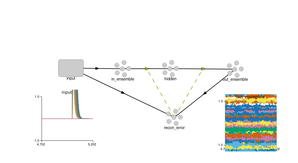
I have set up a simple experiment as described above:
but the input and output vectors look quite different. Is there a way in which I can convert the ensembles into SPA so that I can visualize the dot product against a vocab of all the mnist images? Let me know if this makes sense.
Oh yes. Typo on my part. It should read “it shouldn’t matter”.
Right. The PES is a supervised learning rule, meaning that you’ll need some sort of training signal to tune the weights. This typically means that you’ll also need a target function (that is then used to generate the training signal). It may be possible to re-engineer the autoencoder problem to meet this requirement, because technically the target function is the input you are trying to recreate. The main issue here is how to generate the error signal. If you were just training the output connection (your network is currently training both, adding to the complexity of the problem), using the input weights to generate the training signal might be a viable approach. Here’s a quick setup:
Caveat: This is just a quick thought experiment, I’m not 100% certain this will work.
There is a problem with this approach. The MNIST images (as vectors) don’t really meet the requirements to use with a dot product. Namely, as vectors, the magnitude of the vector isn’t limited to 1, so naively using the dot product will give you erroneous results.
What you could do is to pipe the output of the out_ensemble to a nengo.Node. You can then write custom HTML code that NengoGUI will display (see this example on how to use the _nengo_html_ attribute) to show the flattened vector as an “image”. If you install the NengoExtras repository, there’s a helper function that does all of this for you. You can refer to this example (just ignore all of the FPGA code) to see how to use it.
Once you have the output “vector” displaying as an image, you can then use good ol’ human cognition to judge how well your network is doing.
Thanks! This helped me to see that my auto encoder is actually not learning anything . Looks like it is back to the drawing board for me. I will spend some time to think about this and maybe ask again if I have other additional questions.