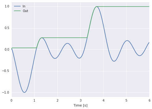
We can improve on Jan’s above solution by adding a scalar transform > 1 to the diff -> peak connection to scale up the difference being integrated. This makes the peak track the input change more quickly.
Assuming no noise in the system (direct mode), and only one level of filtering on the feedback (**), the ideal scaling is 1 / (1 - np.exp(-dt / tau)).
import nengo
import numpy as np


def stim(t):
    return (np.sin(-t - 1.) + np.sin(-3 * t) + np.sin(-5 * (t + 1))) / 3.

with nengo.Network() as model:
    stimulus = nengo.Node(stim)

    peak = nengo.Ensemble(1, 2, neuron_type=nengo.Direct())

    nengo.Connection(stimulus, peak[1], synapse=None)

    tau = 0.1
    dt = 0.001
    a = np.exp(-dt / tau)
    function = lambda x: ((x[1] - x[0]).clip(min=0)) / (1 - a) + x[0]
    nengo.Connection(peak, peak[0], synapse=tau, function=function)

    p_in = nengo.Probe(stimulus, synapse=0.01)
    p_out = nengo.Probe(peak[0], synapse=0.01)


with nengo.Simulator(model) as sim:
    sim.run(6)


import matplotlib.pyplot as plt

plt.figure()
plt.plot(sim.trange(), sim.data[p_in], label="In")
plt.plot(sim.trange(), sim.data[p_out], label="Out")
plt.legend(loc='best')
plt.xlabel("Time [s]")
plt.ylim(-1.1, 1.1)
plt.show()
I’ll give some details on why this works below.
The continuous-time dynamical system that we want to implement is:
$$\dot{x}(t) = f(x(t), u(t)), \quad f(x, u) = \kappa \left[u - x \right]_+$$
where $\left[ \cdot \right]_+$ denotes positive half-wave rectification. $\kappa > 0$ is a time-constant that determines how quickly the state should adjust to the positive difference. Note that in a purely continuous-time system, assuming no noise, $\kappa$ can be made arbitrarily large. Now let’s see what happens when we map this system onto the recurrent population.
Normally we apply Principle 3 to this to get the recurrent function:
$$f’(x, u) = \tau f(x, u) + x = \tau \kappa \left[u - x \right]_+ + x$$
This is what Jan did above (with a subtle difference that will be discussed later (**)) by breaking out the first term into a separate population that is good at decoding the rectification. Jan also implicitly used $\kappa = \tau^{-1}$ by setting a transform of 1 on diff -> peak, which is much smaller than the ideal.
However, I said earlier it’s ideal to have $\tau \kappa = (1 - e^{-dt / \tau})^{-1}$ – not an arbitrarily large constant. This is because our simulation isn’t actually continuous. Since we have discrete time-steps, our desired dynamical system is:
$$x[k + 1] = \bar{f}(x[k], u[k]), \quad \bar{f}(x, u) = \bar{\kappa} \left[u - x \right]_+ + x$$
where $0 < \bar{\kappa} \le 1$ is a discrete time-constant (it is dimensionless). Note that $\bar{\kappa} = 1$ will give a perfect peak detector, assuming no noise.
Now the discrete version of Principle 3 says the recurrent function should be:
$$\bar{f}’(x, u) = (1 - a)^{-1} (\bar{f}(x, u) - ax) = (1 - a)^{-1} \bar{\kappa} \left[u - x \right]_+ + x$$
where $a = e^{-dt/\tau}$. The proof is in my comp-II report – also more information here for the linear case. This is the same as before with $\tau \kappa$ substituted for $(1 - a)^{-1} \bar{\kappa}$. This establishes the ideal gain mentioned previously, when $\bar{\kappa} = 1$.
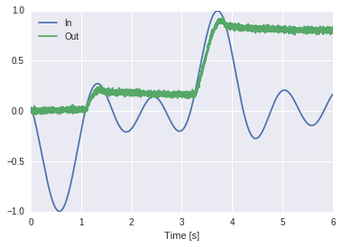
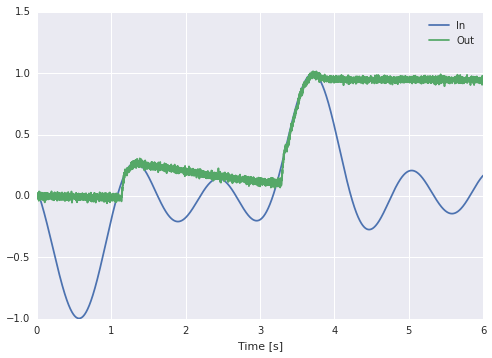
However, when using neurons, this ideal gain will amplify the noise, and so $\bar{\kappa}$ should bet set using a $\texttt{timescale}$ over which to track the input in which the noise will become negligible, i.e. $\bar{\kappa} = dt / \texttt{timescale}$. Then set the transform to dt / timescale / (1 - np.exp(-dt / tau)). In the code below, we “guess” a timescale of $10,\text{ms}$.
As a sanity check, we can note that:
$$\lim_{dt \rightarrow 0} \frac{dt}{1 - e^{-dt/\tau}} = \tau$$
which gives us back the result from the continuous version of Principle 3, with $\kappa = \texttt{timescale}^{-1}$. In other words, we aren’t exploiting the discrete nature of the simulation – dt can still be whatever we want – rather we are properly accounting for the time-step and understanding how it relates to all constants involved.
(**) There is one more subtle thing going on… The above code and the assumption made by standard Principle 3 is that the feedback is only filtered by one lowpass. However, Jan’s code uses two synapses in the part of the feedback that computes $\left[u - x \right]_+$: a synapse of 0.005 on peak -> diff and 0.005 on diff -> peak. A better approximation is to set both of these to tau / 2. I have some theoretical justification for this choice (assuming the noise contributed by each population is equal, and the input derivative is near zero). There is also a more principled approach that is a bit more complicated, but this seems to work well enough.
import nengo
import numpy as np

np.random.seed(0)


def stim(t):
    return (np.sin(-t - 1.) + np.sin(-3 * t) + np.sin(-5 * (t + 1))) / 3.

with nengo.Network() as model:
    stimulus = nengo.Node(stim)
    diff = nengo.Ensemble(
        100, 1,
        intercepts=nengo.dists.Exponential(0.15, 0., 1.),
        encoders=nengo.dists.Choice([[1]]),
        eval_points=nengo.dists.Uniform(0., 1.))
    peak = nengo.Ensemble(100, 1)

    tau = 0.1
    timescale = 0.01
    dt = 0.001
    nengo.Connection(stimulus, diff, synapse=tau/2)
    nengo.Connection(diff, peak, synapse=tau/2, transform=dt / timescale / (1 - np.exp(-dt / tau)))
    nengo.Connection(peak, diff, synapse=tau/2, transform=-1)
    nengo.Connection(peak, peak, synapse=tau)

    p_in = nengo.Probe(stimulus, synapse=0.01)
    p_out = nengo.Probe(peak, synapse=0.01)


with nengo.Simulator(model) as sim:
    sim.run(6)


import matplotlib.pyplot as plt

plt.figure()
plt.plot(sim.trange(), sim.data[p_in], label="In")
plt.plot(sim.trange(), sim.data[p_out], label="Out")
plt.legend(loc='best')
plt.xlabel("Time [s]")
plt.show()