Hmm so this is quite the nice challenge!
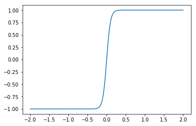
The hard part of the problem comes from the fact that the feedback needs to compute the term np.tanh(x / beta). If we plot this, we see that it has a fairly sharp transition from -1 to +1 around 0…
By default, Nengo distributes the tuning curves uniformly about the space, and so they are not optimized to accurately compute such functions. With the defaults, you would likely need tens of thousands of neurons to approach the level of accuracy that you need to get the dynamics that you want.
Fortunately, there is a way. The most straight-forward approach is to place all of the tuning curves for the x-coordinate so that they “turn on” at x=0. This point is known as the intercept of each neuron.
from nengo.utils.ensemble import tuning_curves

with nengo.Network() as model:
    x = nengo.Ensemble(
        n_neurons=50, dimensions=1, intercepts=np.zeros(50))

with nengo.Simulator(model) as sim:
    plt.plot(*tuning_curves(x, sim))

plt.ylabel("Firing rate (Hz)")
plt.xlabel("Input scalar, x")
plt.show()
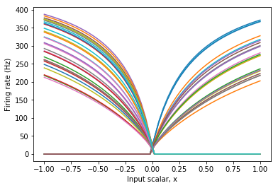
As seen above, this provides tuning curves that more closely match the overall shape of the desired function. Consequently, this ensemble may compute the function with much greater accuracy with fewer numbers of neurons.
To make this work, we now need two separate ensembles, one for the x-coordinate and one for the y-coordinate. We can separate them out because there are no nonlinear interactions between coordinates. We now need 4 separate connections, such that their addition computes the same feedback function as before.
Here is my revised code:
import nengo
import numpy as np
import matplotlib.pyplot as plt
I =.5
epsilon=.2
gamma=6.0
beta=0.1
syn=0.1
n_neurons = 500
neuron_type = nengo.LIFRate()
syn_probe = 0.01
net = nengo.Network(label='Relaxation Oscillator')
with net:
inp = nengo.Node(I)
oscillator_x = nengo.Ensemble(
n_neurons=n_neurons, dimensions=1, neuron_type=neuron_type,
radius=2, intercepts=np.zeros(n_neurons))
oscillator_y = nengo.Ensemble(
n_neurons=n_neurons, dimensions=1, neuron_type=neuron_type,
radius=7)
'''
# osc to osc connection
def feedback(x):
x,y = x
dx = 3 * x - x**3 + 2 - y
dy = epsilon * (gamma * (1 + np.tanh(x / beta)) - y)
return [syn*dx+x,syn*dy+y]
'''
nengo.Connection(oscillator_x, oscillator_x, synapse=syn,
function=lambda x: syn*(3*x - x**3 + 2) + x)
nengo.Connection(oscillator_x, oscillator_y, synapse=syn,
function=lambda x: syn*(epsilon * (gamma * (1 + np.tanh(x / beta)))))
nengo.Connection(oscillator_y, oscillator_x, synapse=syn,
function=lambda y: syn*(-y))
nengo.Connection(oscillator_y, oscillator_y, synapse=syn,
function=lambda y: syn*(epsilon * (-y)) + y)
# inp to osc connection
nengo.Connection(inp, oscillator_x, transform=syn, synapse=syn)
x_pr = nengo.Probe(oscillator_x, synapse=syn_probe)
y_pr = nengo.Probe(oscillator_y, synapse=syn_probe)
with nengo.Simulator(net) as sim:
sim.run(40)
t = sim.trange()
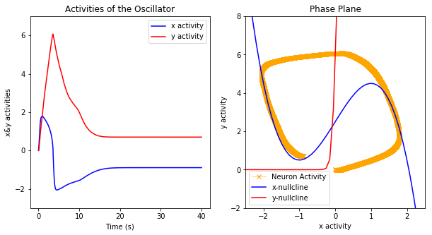
# xy activities
fig1 = plt.figure(figsize=(10, 5))
ax1 = fig1.add_subplot(1, 2, 1)
ax1.plot(t, sim.data[x_pr], label="x activity", color='b')
ax1.plot(t, sim.data[y_pr], label="y activity", color='r')
ax1.set_title("Activities of the Oscillator")
ax1.set_xlabel("Time (s)")
ax1.set_ylabel("x&y activities")
ax1.set_ylim(-3, 7)
ax1.legend()
# phase plane
xmin, xmax, ymin, ymax = -2.5, 2.5, -2, 8
ax2 = fig1.add_subplot(1, 2, 2)
ax2.plot(sim.data[x_pr], sim.data[y_pr], label="Neuron Activity", color='#ffa500', linewidth=.5, marker='x')
X = np.linspace(xmin, xmax)
ax2.plot(X, 3. * X - X ** 3 + 2 + I, label='x-nullcline', color='b')
ax2.plot(X, gamma * (1 + np.tanh(X / beta)), label='y-nullcline', color='r')
ax2.set_title("Phase Plane")
ax2.set_xlabel("x activity")
ax2.set_ylabel("y activity")
ax2.set_ylim(ymin, ymax)
ax2.set_xlim(xmin, xmax)
ax2.legend()
plt.show()
Some further optimizations should be possible. For instance, note that we only need the positive portion of the y space, and so half the space is currently wasted. This could be solved by shifting the space to be centered around 0 and cutting the radius in half.
There may also be a better choice or mix of tuning curves for the x ensemble that is better optimized to accurately compute both np.tanh(x / beta))) and 3*x - x**3 + 2 simultaneously. Solving this sort of optimization problem in general is very difficult (it is a nonlinear optimization problem with discontinuous gradients), and so Nengo currently leaves this as a problem for the user.

 . I guess it means that I do have the correct code, but if I want to use LIFRate, I will have to play around its properties…?
