For nengo.Ensembles in which you connect to the ensemble, and not the ensemble’s neurons, they are running in “NEF-mode”. Conceptually, the computation performed by a NEF ensemble can be broken down into three phases: encoding, the neuron non-linearity, and decoding.
The encoding phase converts the post-synaptic vector value (which is specified by the nengo.Connection, which is a separate object) into the input current for the neuron. For nengo.Ensembles, the encoders and normalize_encoders initialization parameters are used in this phase. The dimensions parameter is also indirectly used here since that determines the dimensionality of the encoders.
The neuron non-linearity phase takes the input current and puts it through the neuron non-linearity to figure out if a spike should occur or not. For nengo.Ensembles, the intercepts, max_rates, gain, bias and neuron_type initialization parameters are used to determine the shape and response of the neuron non-linearity used for this phase.
The decoding phase converts the spikes (or firing rates for rate-mode neurons) back into vector space. For nengo.Ensembles, the eval_points initialization parameter is used in this phase to compute the decoders for this ensemble.
For parameters involved in the encoding and neuron non-linearity phase of the computation, it is assumed to be specified using a unit vector basis. This means all values are assumed to be specified within a range of -1 to 1. For the parameters in the decoding phase, it is assumed to be specified using the radius basis, i.e., specified within the range of -radius to radius.
Now let’s understand what the radius parameter does, and why it is needed. Since the encoding and neuron phases of the ensemble computation assume a unit vector basis, there is an issue that arises when the user wants to get the ensemble to represent values that are greater than the unit vector. If the user simply feeds the raw input vector into the ensemble, the neurons would saturate, and the representation by the neuron would not be very accurate. So, what can the user do? The obvious solution is to scale the input vector by some fixed value before feeding it to the ensemble. The scaling value would have to be chosen such that for all expected input values, the value being passed to the neuron (i.e., post scaling) would be within this -1 to 1 range. But if the user applies this scaling value on the input, they’ll also need to apply the same scaling value on the output in order for there to be no effective change to the vector values being represented by the ensemble. Requiring the user to do this (both the input and output scaling) is tedious, and non-intuitive, so we introduced the radius parameter as a shortcut that handles this scaling for you.
So, how does this affect your tuning curve? If you specify the intercepts for your neurons to be at 0.5, Nengo will set the intercepts for your neurons to be at 0.5, using a unit basis. If we set the radius to be a non-unit value, the input scaling done by the radius changes the effective value of the intercept. As an example, if the radius was set to 10, all inputs to the ensemble would be scaled by 1/10 before being processed by the neuron non-linearity. Thus, for the neuron’s input current to be 0.5 (i.e., where the intercept is), the vector input would have to be 5 (i.e., 0.5 * 10), which is what you observe in your graph.
This is another consequence of how the ensemble computation is split up into the three conceptual parts. If you look at it closely (as we will in a bit), you will see that the negative intercept actually is being respected by the Nengo code.
Recall how I described the neuron non-linearity phase above. I mentioned that in this phase, the computations are being done in the neuron “current” phase, where values here are analogous to currents in real neurons. Since all of the neurons in the ensemble are of the same type, you’d expect that the neurons will reach their maximum firing rate either going in the positive x direction, or in the negative x direction. For LIF neurons, the firing rate of neurons always increases in the positive x direction.
When you define an intercept for a neuron, it will respect this convention, where positive x denotes an increase in input current. Note that a negative x value doesn’t necessarily mean negative current, because there are bias currents that are not outwardly visible to the user – remember that in this space, everything is just normalized to be between -1 and 1.
Okay, so how does this explain what you see in your tuning curve plot? The tuning curve plots the ensemble’s response to inputs in vector space. This means that it takes the neuron’s encoders into account when making this plot. The second neuron in your ensemble has an encoder of [-1], which means that it is more active as the input vector goes in the -x direction. But, recall that the intercepts are defined in the neuron current space, which means that the intercept you see on the tuning curve must take into account the neuron’s encoder. For the first tuning curve plot (where radius==1), you specified the intercept of the second neuron to be -0.5. The question is, for what input vector value does the second neuron reach this intercept in current space?
Let’s choose a random input vector, say [0.2]. After the encoding phase, this input vector gets turned into a current value by multiplying it with the neuron’s encoder. The current value being passed to the neuron’s non-linearity is then np.dot([0.2], [-1]) = -0.2. So… for what input vector value does the neuron’s current equal -0.5 (which is the intercept)? Doing the reverse calculation, we see that it’s 0.5, which is exactly what we see in the tuning curve plot! Essentially, the minus sign in the encoder and the minus sign in the intercept value have cancelled out, resulting in the tuning curve plot you see.
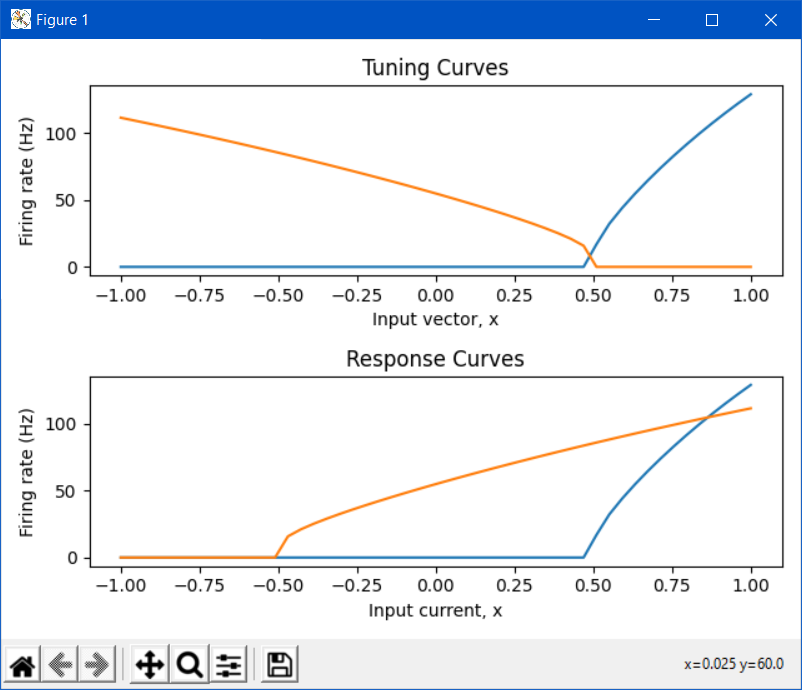
If you want to plot the neuron’s response in the neuron’s current space, what you’ll want to use is the response_curve function. When you use this function to plot the ensemble’s response curve, it ignores all of the encoders. The following plot compares the tuning curve vs the response curve for the network you provided above:
As a side note:
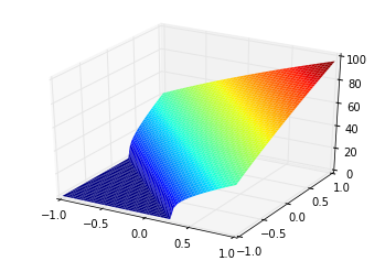
We use the term “tuning curve” and “response curve” to differentiate the vector-based tuning (i.e., a neuron can be thought to be “tuned” to be sensitive to a certain input vector), and the current-based response (i.e., a neuron can be thought to be “responding” to an input current stimulus) of the ensemble of neurons. Also note that the tuning curve doesn’t have to be constrained to 1D, and can be used for multi-dimensional ensembles (although, the most you can plot is 2D, since the tuning curves for a 2D ensemble is a 3D plot). This is an example of a tuning curve for one neuron in a 2D ensemble (taken from @tcstewar’s course notes for the NEF course, available here!):